Today we will look at how to plot a function graph, Excel will help us with this. We will also briefly review some other useful features of the spreadsheet editor.
Application
So, let's move on to solving the question of how to build a function in Excel. This spreadsheet editor is an excellent tool for work in the office and at home. Excel is perfect for calculating your expenses or making serious financial conclusions about the work of a large company. The spreadsheet editor has many features, but today we will talk about one of the most popular ones.
Plotting
We can build a graph of a function in Excel of the usual type or related to the most complex mathematical operations. To do this, we perform several steps. Open a blank Excel sheet or start a new project. We create two columns. Further in the first we write down the argument. We directly enter the functions in Excel in the second column. Let's move on to the next step. We indicate in the first column the X values necessary for the calculation, as well as plotting. We define the segment within which the function will be created. 
Payment
Let's move on to the next column. It is necessary to write the formula of the Excel function in it. The graph will be built on its basis. All spreadsheet formulas start with the "=" sign. The application features greatly simplify the process of creating a graph. For example, you do not need to enter the selected formula in all rows. The developers of Excel took into account that this would not be very convenient. So, we just stretch the formula, and it will be built in each of the cells. You just need to click on the appropriate area. 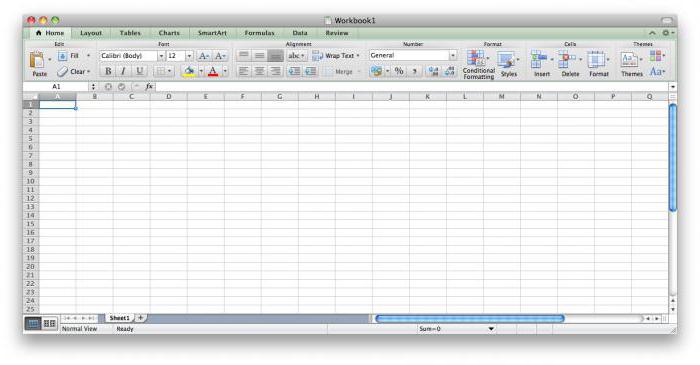
Stretch Details
We continue the process of building a function in Excel. After completing the steps above, a small square will appear in the lower right corner of the cell. Move the cursor over it so that its pointer changes. Now we clamp right button mouse and stretch the formula to the required number of cells. As a result, such actions will help create a graph of the Excel function. 
Instruction
We proceed directly to the construction. In the "Menu" select the "Insert" tab. In the list of proposed options, use the "Diagram" item. Select any of the available scatter plots. We press "Next". We need a scatter plot. Now we will tell you why. Other diagrams will not allow you to create in a single and argument. The value view uses a reference to the desired group of cells. As a result of the actions taken, a new dialog box will appear, in it we press the "Row" button. 
Let's move on to the next step. Create a row using the "Add" button. The following window will appear, in which we set the search path for the required values to build the required graph. In order to select the desired cells, click on the thumbnail image Excel tables. Specify the required cells in the table. Soon the required function will appear on the sheet, the value in Excel has already been set, and all that remains is to click Finish. The chart has been built. If desired, it can be of any size and complexity.
Other features
We have dealt with the issue of constructing functions and graphs for them, however, the spreadsheet editor has a number of other features that you should also be aware of to make working with it easier. Speaking about the mathematical capabilities of Excel, one cannot ignore the subtraction function. To calculate the difference between two numbers, click on the cell where the result will be displayed. Enter the equal sign. If the content begins with this symbol, Excel thinks that a certain mathematical operation or formula has been placed in the cell. After the mentioned equal sign, without using a space, we type the number to be reduced, put a minus and enter the subtrahend. After that, press Enter. The cell will display the difference between the two numbers.
Consider a variant in which the initial data must be taken from other cells of the table. For example, in order to show the number in cell D1 reduced by 55 in cell B5, click on B5. Enter the equal sign. After that, click on cell D1. The equal sign will be followed by a reference to the cell we have chosen. You can also type the desired address manually without using the mouse. After that, enter the subtraction sign. Specify the number 55. Press Enter. Excel will then automatically calculate and display the result.
In order to subtract the value of one cell from the indicators of another, we use a similar algorithm. Enter the equal sign. We type the address or click the cursor on the cell in which the value to be reduced is located. After that, we put a minus. Enter or click on the cell containing the value to be subtracted. We use the Enter key. Action completed.
It has already been noted above that formulas are used to build a function in Excel, so you should get acquainted with the features of their creation. There are a number of specific rules for this. Among other things, formulas allow you to automate the process of calculating values entered into cells. Let's start from the very beginning. We start Excel. Let's take a closer look at the familiar interface. The formula bar is labeled fx. She is what we need.
To enter a simple formula, specify the desired value in the cell by entering an equal sign in front of it. After pressing the Enter key, we will see the result. There are several ways to enter data. Click on the empty cell A1. We insert a certain value into it, prefixing it with the “equal” symbol. We pass to the next cell B1. We specify in it another element of the formula. We continue similar actions until all the parameters provided in the task are entered into the table. We put the "equal" sign in the last empty cell.
Let's move on to the next step. Select cell A1. We insert an arithmetic sign into it (division, multiplication, addition). Select another cell, for example, B2. Press Enter. We create the original expression by double-clicking on the cell and pressing Ctrl and "Apostrophe".
So we figured out how to plot the Excel function, and also studied the principle of working with formulas and algorithms that may be required for this.
Lesson Objectives:
- teach how to plot elementary graphs mathematical functions using an Excel spreadsheet;
- show the possibilities of using Excel to solve problems in mathematics;
- to consolidate the skills of working with the Chart Wizard.
Lesson objectives:
- educational– familiarization of students with the basic techniques for plotting function graphs in Excel;
- developing- the formation of students' logical and algorithmic thinking; development of cognitive interest in the subject; development of the ability to operate with previously acquired knowledge; development of the ability to plan their activities;
- educational- education of the ability to think independently, responsibility for the work performed, accuracy in the performance of work.
Lesson type:
- combined
Tutorials:
Computer science. Basic course 2nd edition / Ed. S.V. Simonovich. - St. Petersburg: Peter, 2004.-640s.: ill.
Hardware and software:
- Personal computers;
- Windows application- Excel spreadsheets.
- Projector
Handout:
- Cards with individual tasks for plotting function graphs.
Lesson plan.
- Organizational moment - 3 min.
- Checking homework -10 min.
- Explanation of new material – 20 min.
- Application of acquired knowledge – 20 min.
- Independent work. - 20 minutes
- Summing up the lesson. Homework - 7 min.
During the classes
Organizing time
Checking students' readiness for the lesson, marking absentees, announcing the topic and objectives of the lesson
Checking homework. (front poll)
Questions to check
- What is a workspace Excel programs?
- How is the cell address determined?
- How to change column width, row height?
- How to enter a formula in Excel?
- What is a fill marker and what is it for?
- What is relative cell addressing?
- What is absolute cell addressing? How is she asked?
- What are headers? How are they asked?
- How to set the margins of a printed document? How to change paper orientation?
- What is the functional dependence y \u003d f (x)? Which variable is dependent and which is independent?
- How to enter a function in Excel?
- What is the graph of the function y \u003d f (x)?
- How to build a chart in Excel?
Explanation of new material.
When explaining new material can be used excel file with task templates (Appendix 1), which is displayed on the screen using a projector
Today we will consider the use of an Excel spreadsheet processor for function graphs. In the previous practice, you have already built diagrams for various tasks using the Diagram Wizard. Function graphs, as well as charts, are built using the Excel Chart Wizard.
Consider the construction of graphs of functions using the example of the function y \u003d sin x.
View this chart well known to you from math lessons, let's try to build it using Excel.
The program will build a graph by points: points with known values will be smoothly connected by a line. These points need to be specified to the program, therefore, first a table of function values \u200b\u200bis created y \u003d f (x).
To create a table, you need to define
- segment of the x-axis, on which the graph will be built.
- step variable x, i.e. over what interval the values of the function will be calculated.
Task 1. Plot the function y \u003d sin x on the segment [- 2; 2] with step h = 0.5.
1. Fill in the table of function values. In cell C4, enter the first value of the segment: - 2
2. In cell D4, enter a formula that will add a step to the left-standing cell: = B4 + $A$4
3. Fill cell D4 to the left with the fill marker of row 4, until we get the value of the other end of the segment: 2.
4. Select cell C5, call the Function Wizard, select the SIN function in the mathematical category, select cell C4 as the function argument.
5. Use the fill marker to spread this formula in the cells of row 5 to the end of the table.
Thus, we got a table of arguments (x) and values (y) of the function y \u003d sin x on the segment [-2; 2] with a step h \u003d 0.5:
| x | -2 | -1,75 | -1,5 | -1,25 | -1 | -0,75 | -0,5 | -0,25 | 0 | 0,25 | 0,5 | 0,75 | 1 | 1,25 | 1,5 | 1,75 | 2 |
| y | -0,9092 | -0,9839 | -0,9974 | -0,9489 | -0,8414 | -0,6816 | -0,4794 | -0,2474 | 0 | 0,2474 | 0,4794 | 0,6816 | 0,8414 | 0,9489 | 0,9974 | 0,9839 | 0,9092 |
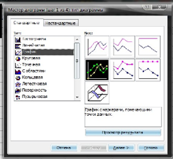
6. Next step. Select the table and call the Chart Wizard. At the first step, select Non-Standard Smooth Graphs in the tab.
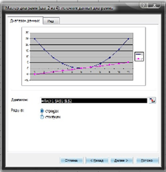
7. On the second step in the Row tab, do the following:
In the Row field, select the x row and click on the “Delete” button (we don’t need a graph of changes in x. A function graph is a graph of changes in y values)
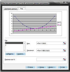
Click the button in the X-Axis Labels field. Select cells with x values in the table and click the button. The labels on the horizontal axis will become the same as in our table.
8. In the third step, fill in the Headings tab.

9. An example of the resulting graph.
In fact, so far this has little resemblance to a function graph in our usual sense.
To format a graph:
- Let's call the context menu of the y-axis. Then, select Format Axis…. In the Scale tab, set: the price of the main division: 1. In the Font tab, set the font size to 8pt.
- Let's call the context menu of the OX axis. Select Format Axis….
In the Scale tab, set: intersection with the y-axis, set the category number 5 (so that the y-axis intersects the x-axis in the category labeled 0, and this is the fifth category in a row).
In the font tab, set the font size to 8pt. Click on the OK button.
The rest of the changes are made in the same way.
To consolidate, consider another task for plotting a graph of functions. Try to solve this problem yourself, referring to the projector screen.
Application of acquired knowledge.
Invite a student to the projector and formulate the following task.
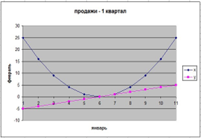
Task 2. Construct a graph of the function y \u003d x 3 on the segment [- 3; 3] with step h = 0.5.
1. Create the following table: Create a table of function values y = f(x).

2. In cell C4, enter the first value of the segment: -3
3. In cell D4, enter a formula that will add a step to the left-standing cell: = B4 + $A$4
4. Fill cell D3 to the left with the cell fill marker 3 until the value of the other end of the segment is obtained: 3.
5. In cell C5, enter the formula for calculating the value of the function: = C4 ^ 3
6. Use the fill marker to copy the formula into the cells of line 5 to the end of the table.
Thus, a table of arguments (x) and values (y) of the function y \u003d x 3 on the interval [–3; 3] with a step h \u003d 0.5 should be obtained:
| X | -3 | -2,5 | -2 | -1,5 | -1 | -0,5 | 0 | 0,5 | 1 | 1,5 | 2 | 2,5 | 3 |
| y | -27 | -15,625 | -8 | -3,375 | -1 | -0,125 | 0 | 0,125 | 1 | 3,375 | 8 | 15,625 | 27 |
7. Select the table and call the diagram wizard. In the first step, select Smooth Graphs in the second tab.
8. On the second step, in the Row tab, perform:
9. At the third step, fill in the Headings tab.

10. An example of the resulting graph:
11. Draw up a schedule.
12. Set page options and chart sizes so that everything fits on one landscape sheet.
13. Create headers and footers for this sheet (View Headers and Footers...):
14. Header on the left: graph of the function y = x 3
Independent work.
Work on cards with individual tasks. (Annex 2)
An example of a card, with a general task, is displayed on the screen using a projector.
1. Plot the function y=f(x) on a segment with a step h=c
2. Set the page settings and chart dimensions so that everything fits on one landscape sheet.
3. Create headers and footers for this sheet (View Headers and Footers...):
- Header on the left: graph of the function y=f(x)
- footer in the center: your full name and date
After completing the task, the correctness of each option is checked using a projector.
Summarizing.
Homework.
Lesson grades.
Function calculation technology in EXCEL . Graphing Technology
The rapid development of computer technology, information and communication technologies has led to the fact that an increasing number of people use computers not only to perform their official duties at work, but also at home, in everyday life. Everyone uses computers: schoolchildren, students, employees and heads of firms and enterprises, scientists.
Computers are most widely used for solving office tasks: typing and printing texts (from simple letters and abstracts to serious scientific papers consisting of hundreds of pages and containing tables, graphs, illustrations), calculations, working with databases.
Historically, the vast majority of users work in operating system Microsoft Windows and for solving office problems use the package Microsoft office. And this is not surprising, because the programs included in the package allow you to solve almost any problem. In addition, Microsoft is constantly working on improving its software products, expanding their capabilities, making them more convenient and friendly.
Microsoft Excel is a spreadsheet (quite often referred to simply as a "spreadsheet") computer program designed to perform economic, scientific and other calculations. Using Microsoft Excel, you can prepare and print, for example, a statement, invoice, payment order, and other financial documents.
With help from Microsoft Excel can not only perform calculations, but also build a chart.
Microsoft Excel is an indispensable tool for preparing various documents: reports, projects. Tables and charts created in Microsoft Excel.
In Microsoft Excel, you can paste, for example, into text typed in Microsoft Word, or to a presentation created in Microsoft Power Point.
Functions are designed to make it easier to create and interact with spreadsheets. The simplest example of performing calculations is the addition operation. Let's use this operation to demonstrate the advantages of functions. Without using the system of functions, you will need to enter the address of each cell separately into the formula, adding a plus or minus sign to them. As a result, the formula will look like this:
B1+B2+B3+C4+C5+D2
It is noticeable that it took a lot of time to write such a formula, so it seems that it would be easier to calculate this formula manually. To quickly and easily calculate the sum in Excel, you just need to use the sum function by clicking the sum sign button or from the Function Wizard, you can also manually type the function name after the equal sign. After the name of the functions, you need to open a bracket, enter the addresses of the areas and close the bracket. As a result, the formula will look like this:
SUM (B1:B3; C4:C5; D2)
If we compare the notation of formulas, we can see that the colon here denotes a block of cells. Function arguments are separated by a comma. Using blocks of cells, or areas, as arguments for functions is advisable, since, firstly, it is clearer, and secondly, with such a record, it is easier for the program to take into account changes on the worksheet. For example, you need to calculate the sum of the numbers in cells A1 to A4. This can be written like this: =SUM(A1;A2;A3;A4) Alternatively: =SUM(A1:A4)
Functions - these are built-in Excel formulas that perform complex mathematical calculations.
Functions in Excel calculate values and are used in cases where the data cannot be obtained in any other way, and also when complex calculations need to be made, and creating a formula from scratch is time consuming.
With all the variety of functions in Excel and the possibility of combining more complex formulas, it is difficult to consider absolutely all options.
Composition of functions
A function consists of a name and arguments enclosed in parentheses. A function can have multiple arguments (must be separated by commas) or none.
Table 1 shows some examples.
Table 1
Entering functions
The easiest way to enter a function is to click on the button Insert function in the formula bar and select the one you need in the dialog box Function Wizard - step 1 of 2 ( Picture 1 ) .
Rice. one
If you do not know which function to use, enter a brief description of its actions in the field Function search and click on the button Find .
After selecting a function, click on the button OK. A dialog box will appear Function arguments ( Figure 2 ) A that allows you to enter the arguments to the function.
This window will display their current values.
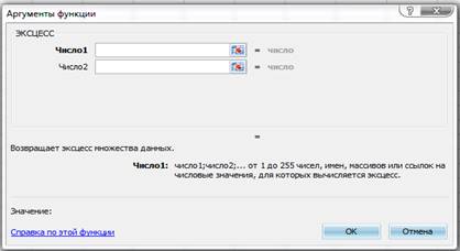
Rice. 2
If you know the name of the desired function, you can enter it directly into the formula. If they know how to use arguments, they enter opening quotes, a list of arguments, closing quotes.
nested functions
A formula can consist of a single function like =DATE() or
\u003d REV (123.65). However, often in one function, in addition to references to cells and ranges, other functions are used as an argument. For example: =ABS (SUM(C2:C20)) .
Here the function SUM sums the values in the cells with C2 on C20. This value becomes the argument to the ABS function, which returns the absolute value of the sum. You can create complex functions with up to seven levels of nested functions.
Using the IF Function
Function IF absolutely necessary for creating dynamic worksheets. Here is the basic form: IF (logical expression; value if true; value if false) .
First function argument IF- boolean expression
matter True or Lie. Such values have, for example, expressions AT 9<6 - cell value B9 less than 6, aQ10<>R15 – Q10 not equal to R15 .
The next two arguments determine what value the function returns. IF. If the boolean expression is True, the function returns true; if the boolean expression has a value Lie, the function returns false. Return values can be both text and numeric.
For example: =IF((R11+S11)>0; (R11+S11)*Q4; "N/A") .
Formula places text "There is no data" into a cell if the sum of the values
in cells R11 and S11 equal to or less 0 . If not, the cell will contain the number value.
This example is schematic. Operator IF becomes a very powerful tool when used with changing values and other functions. In practice, this function is called very often.
Overview of Excel Functions
There are too many functions in Excel, and it would take too long to go through each of them in detail. Therefore, below is a brief tour of computing power at your disposal.
Let's get acquainted with some of the features of the proposed functions - this will save a lot of time: without creating your own formulas, you can achieve the same results using built-in functions.
It must be remembered that Excel has a much greater variety of functions.
Information functions (see Table 2) allow you to find out about the type of data stored in cells.
table 2
| FUNCTION | RETURN VALUE |
| CELL | User-defined information about a given cell (values, format, variable type, or color) |
|
EMPTY |
Number of empty cells in the selected range |
| INFO | Accurate computer information (size random access memory, equipment, etc.) |
| EMPTY | True if the specified cell is empty |
| ISNUMBER | True if the specified cell contains a number |
| ETEXT | True if the specified cell contains text |
| TYPE OF | A number representing the type of values contained in the specified cell |
An important group of functions are the logical functions (see Table 3).
Table 3
The date and time functions (see Table 4) allow you to create formulas that perform calculations based on time and date, as well as perform calculations with dates. Excel uses special numbers (date values) to store and manipulate dates. To convert regular dates to values used in Excel, you can use the function THE DATE. Functions DAY , YEAR and MONTH convert date values to human readable values.
Table 4
| FUNCTION | RETURN VALUE |
| THE DATE | Common date entry value to values used in Excel |
| DAY | Integer variable corresponding to the day of the month (similar functions: YEAR , MONTH , HOUR , MINUTES AND SECONDS) |
| TODAY | Date and time value on PC. Use TODAY to return only the date and TIME- only time |
| DAYWEEK | Day of the week |
| WORKDAY | The date of the next business day after the specified |
| SHARE YEAR | A decimal fraction representing the fraction of a year equal to the interval between dates. Convenient to use for calculating employee bonuses |
The search and link functions (see Table 5) specify cells in a worksheet range or values in an array. Functions from the database category are auxiliary, they are convenient to use if the worksheet is correctly formatted.
Table 5
The math and trigonometric functions (see Table 6) perform mathematical calculations.
Table 6
| FUNCTION | RETURN VALUE |
| ABS | Argument modulus |
| COS | The cosine of the argument. Excel has a full set of trigonometric functions |
| FACT | Factorial of the argument |
| LOG | The logarithm of the argument (use LN to get the natural logarithm) |
| PI | Number PI |
| PRODUCTS | The product of all arguments (you can specify a range of cells, as is the case with the function SUM) |
| ROMAN | Roman numerals |
| ROUND | Rounded value to the specified number or decimal place |
| SIGN | 1 - if the argument is positive, 0 - if equal to zero, -1 - if the argument is negative |
| ROOT | The square root of the argument |
| SUMPRODUCT | Multiplies the corresponding elements in two or more arrays and then sums the results |
| WHOLE | The integer part of the argument - the part after the decimal point is discarded |
Text functions (see Table 7) cast text variables to the desired form or display text based on numeric arguments.
Table 7
| FUNCTION | RETURN VALUE |
| All non-printable characters are removed from the text | |
| RUBLE | Converts a numeric value to text, in currency format, with two decimal places |
| LEFT | The specified number of characters to the left of the string ( PSTR and RIGHT select characters from the center or right side of the input string) |
| DLSTR | Number of characters per line |
| LOWERLINE | String text is converted to lowercase |
| TEXT | Turns numbers into corresponding text, patterned |
| TRIM | Removes extra spaces(single spaces between words preserved) |
Because Excel's main job is to help you do business, it contains hundreds of functions for calculating debt, investments, and similar economic values (see Table 8).
Table 8
| FUNCTION | RETURN VALUE |
| ACCRINT | Calculating interest rates on interest payable |
| PS | Returns the present value of an investment |
| DISCOUNT | Returns the discount rate for a security |
| BS | Return on investment at constant interest rate |
| INORMA | Returns the interest rate for a fully invested securities |
| HPMT | The amount of interest payments on investments or debts |
| INCOME | Income from securities |
| PMT | Returns the amount of the periodic payment |
| CHISTNZ | Net present value of investment |
| INCOME | Interest rate charges |
About 80 Excel statistical functions are used not for mathematical calculations, but for statistical analysis of any complex data (Table 9). Below are some of the existing functions that will be useful even to ardent fans of mathematical calculations.
Table 9
| FUNCTION | RETURN VALUE |
| AVERAGE | Arithmetic mean of arguments |
| HI2TEST | Data independence test based on chi-square distribution |
| TRUST | Population Confidence Interval |
| CHECK | Number of cells in the specified range that contain numeric values |
| FISHER | Fisher transform |
| FREQUENCY | An array containing the limits in which values change |
| GREATEST | Value in special sequences (to determine, for example, the third largest CDs in the third quarter). LEAST gives the opposite result |
| MAX | The largest value in the sequence. MIN gives the smallest value |
| MEDIAN | Median of argument |
| MORE | Most common value |
| NORMDIST | Normal distribution |
| STDEV | Standard Deviation Estimation |
Many people use Excel as a database manager simple files(without references), storing data in rows and columns of the worksheet (column is a field and row is a record). There are more than ten functions in the database management category (see Table 10). In most cases, they need to specify a range containing the database, fields, and selection criteria.
Table 10
Definition of named constants
The standard method for defining a constant is to place its value in a cell and refer to that cell when the need arises to use the constant in a formula. When changing a constant, it is enough to enter a new value in the cell, and all dependent results will be calculated automatically.
If the value is truly immutable, you can define a named constant that exists only in Excel's memory, not in a worksheet cell. Choose a team Insert / Name / Assign .
In the dialog box Naming, enter the name of the constant and its value in the field Formula, removing existing values (don't remove the equals sign). In this dialog box, you can view all named constants.
Using Microsoft Excel, you can not only perform calculations, calculate logarithmic, trigonometric functions, and build graphs based on these calculations.
Representation of data in graphical form allows you to solve a wide variety of tasks. The main advantage of such a representation is visibility. The trend is easily visible on the charts. You can even determine the rate of trend change. Various ratios, growth, the relationship of various processes - all this can be easily seen on the graphs.
Graphs are used, as a rule, to display the dynamics of changes in a number of values. They are used to reflect temporal trends.
Chart subtypes
one). Standard schedule;
Graph of the usual type.
2). Graph with accumulation;
A graph with stacked data series.
3). A graph in which data sets are stacked and normalized to 100%;
4). Graph with data markers;
Plot with markers on connection nodes marking data points.
five). Graph with accumulation;
6). Normalized schedule;
7). Volume chart;
Volumetric version of the graph with three coordinate axes.
Non-standard charts:
Smooth graphics;
Graph | bar graph;
A kind of hybrid of a histogram and a graph is a non-standard chart Graph-histogram. It has both.
Graph-histogram 2;
Graphs (2 axes);
Color charts;
Chart Color Charts is very attractive. It is more perfect and refined for visual viewing.
B&W chart and time.
Plotting
To build a graph, run the command Box Diagram or using the Chart Wizard.
Row and column labels called row and column headings. If you do not include line labels in the plotting area, then at the 4th step of plotting you need to specify that 0 rows are allocated for row labels.
Column Labels are the text of the legend. The legend is a rectangle that indicates what color or type of lines the data from a particular line is displayed on a graph or chart.
In Excel, to display charts, you can use not only columns, lines and points, but also arbitrary drawings. When plotting mathematical functions, smooth curves should be used as the chart type.
Excel supports a logarithmic scale when plotting graphs, both for regular types of graphs and for mixed ones, that is, you can enter a logarithmic scale on one axis, and a linear one on the other.
Building with the Wizard
The default chart creation method is handy when it doesn't matter which chart type to use. If the user knows in advance which chart he wants to build, for example, more complex than the one offered by Microsoft Excel by default, then you need to use the Chart Wizard.
The program offers the assistance of a diagram wizard. The Chart Wizard guides you through a four-step procedure, at the end of which you have a completed chart.
Before considering each step of the Chart Wizard, it is necessary to review the set of buttons that are available in each of its dialog boxes.
The set consists of 5 buttons: Help, Cancel,<Назад, Далее>, Ready.
The Help button brings up the Assistant, which will guide you through all the details of creating a diagram.
The Cancel button resets all settings made in the Chart Wizard and closes it. Chart creation stops. The next dialog box of the Wizard will also be closed. You can close the Chart Wizard window at any step using the Close icon on the system bar (x).
Buttons< Назад и Далее >designed to navigate within the Chart Wizard step by step. In the first step, the button< Назад недоступна, так как движение еще на один шаг назад невозможно. На последнем шаге кнопка Далее >is not available, since the fourth step is the last and advancement is impossible. It is not clear why these buttons are there at all, since it is very easy to remove them programmatically.
The Done button is present at every step. If the settings in the following steps are not needed, then it is not necessary to go through them. It is enough to click on the Done button, and the diagram will be built according to the settings that have already been set. If cell ranges are not specified, then the chart will still be built, although it is empty.
Before calling the chart wizard, select the range of cells that contains the information used to create the chart. Keep in mind that in order to achieve the desired results, the information should be presented in the form of a continuous table - then it can be distinguished as a single range.
When creating a graph that uses the X and Y axes (as with most charts), the Chart Wizard usually takes the column headers of the selected table to label the X axis. If the table has row headers, the wizard uses them to label variables (if you want to turn them on). The legend (label) identifies each point, bar, and bar in the chart representing the values of the variables.
If you have selected a range of cells, then you can create a graph.
1. Click the ChartWizard button on the Standard toolbar to open the ChartWizard - Step 1 of 4 - ChartType dialog box. The Chart Wizard button has an icon with a graph. When you click this button, Excel will open the dialog box shown in Fig. 3.
2. To select a different chart type, click the appropriate item in the ChartType list box. To select a different subtype, click its representation in the ChartSubtype area of the dialog box. You can see the selected data as a graph of the selected type if you click (and hold down) the Result View (PressandHoldtoViewSample) at the bottom of the dialog box.
This dialog box allows you to change the range of the data on which the graph should be plotted (or define it if it has not already been done). You can also specify how the data series in this range are represented.
When this dialog box is displayed, the range of cells selected in the table prior to activating the Chart Wizard will be surrounded by a moving dotted line and presented as a formula (with absolute cell coordinates) in the Data Range text box.
If you need to change this range (for example, to include a column header row or a row header column), click the range of cells again with the mouse, or edit the cell coordinates in the Range box.
If, during these manipulations, the dialog box Chart Wizard (step 2 of 4): chart data source obscures the table, you can reduce it to the size of the Range field by clicking on the button with the table icon (this icon is located in the dialog box field).
To restore the dialog box, click this button again.
Keep in mind that the Chart Wizard (Step 2 of 4): Chart Data Source dialog box automatically shrinks to the size of the Range box as you drag the mouse pointer over worksheet cells, and automatically restores when you release the mouse button.
4. Check the range of cells presented in the Range field and, if necessary, correct the cell addresses (either using the keyboard or by selecting cells in the table itself).
Typically, the wizard creates a separate series in the chart based on the values of each column of the marked table. A legend (a rectangular area with sample colors or patterns used by the chart) identifies each row (variable) in the chart.
In terms of the selected data from the table, each column of the chart represents the amount of sales for the month, and these results are collected in several groups corresponding to different companies. Optionally, you can redefine value sets for variables from columns to rows. To do this, in the group of radio buttons Rows in (Seriesin) set the radio button Columns (Rows). In this example, you will group the chart columns so that the company's sales data for each month will be collected together.
Because the chart sequences data by column, the wizard uses the items in the first column for x-axis labels (called category labels). The Chart Wizard applies the elements of the first row to the labels in the legend.
5. If you prefer to have the Chart Wizard generate row-by-row (rather than column-by-column) data sequences, in the Seriesin radio button group, click the Rows radio button.
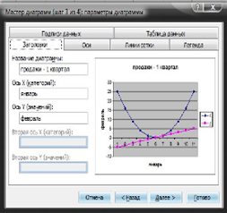
If you want to make individual changes to either the headers or the contents of the cells in the selected range, go to the Series tab of the dialog box (Figure 4) Chart Wizard (Step 2 of 4): Chart Data Source
The dialog box that is displayed (Figure 4) allows you to set a number of options, such as whether the chart should have titles, grid lines, a legend, series labels, and a table with the values from which the chart was created.
7. Depending on the parameters you want to change, select the appropriate tab (Titles, Axes, Gridlines, Legend, DataLabels or DataTable), and then make the necessary changes.
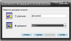
This dialog allows you to place a new graph either on its own sheet in the workbook or as a graphic object on one of the existing sheets in the workbook.
9. To place the chart on its own sheet, select the radio button Separate (Asnewsheet); then, optionally, enter a new sheet name (i.e. replace the suggested Chart1 (Chartl) with something else) in the text field on the right.
To place the chart as an object on one of the existing sheets in the workbook, select the radio button Asobjectin, and then select the sheet name from the drop-down list on the right.
10. Click the Finish button or click
If the Separate radio button is selected, the new chart will be created on its own sheet, and the Chart toolbar will appear on top of it in the workbook window - If the Existing radio button is selected, the new chart will be displayed as an active graphic object on the worksheet sheet in the previously selected area. In addition, the Charts toolbar will magically appear above the worksheet window.
Instant Charts
If you don't have time to complete the four steps above or don't feel like messing around with the Chart Wizard, you can create a complete chart by simply clicking the Finish button in the first window of the Chart Wizard.
You will also create a graph without even opening the Chart Wizard window. Select the desired range of cells and press the key
Using the Charts toolbar
After creating a graph, you can make changes using the buttons on the Charts toolbar.
· Chart elements (Chartobjects). To select a chart element to convert, first click on the Chart Elements drop-down list button, and then click on the name of the object in the list. You can also select an object by clicking on it directly in the diagram. In this case, its name will automatically appear in the list box.
· Format object. To change the format of the selected chart object, the name of which is presented in the field.
· Chart elements, click on the Format button; A dialog box will open with formatting options. Note that the name of this tool, displayed as an on-screen tooltip, changes according to the selected chart object. Therefore, if the edit field of the Chart Elements tool contains a ChartArea, this button will be named Format ChartArea.
· Chart type. To change the chart type, click the down arrow button and select the appropriate chart type from the palette that opens.
· Legend. To hide or show the chart legend, click this button.
· DataTable. Click this button to add or remove the table of data that the chart is based on.
By rows (ByRow). Click this button to have the data series in the chart represent rows of values in the selected data range.
By columns (ByColumn). Click this button to have the data series in the chart represent the columns of values in the selected data range.
Text is clockwise. If the Category Axes or Value Axes objects are selected on the diagram, clicking on this button will allow you to rotate the rows of labels of these objects by 45 clockwise (as the letters a, b are rotated on the button icon).
· Anglecounterclockwise text. If Category Axes or Value Axes objects are selected on the diagram, clicking on this button will allow you to rotate the rows of labels of these objects by 45 counterclockwise (as the letters a b on the button icon are rotated).
Graph editing
Sometimes it may be necessary to make changes to certain parts of the graph (choose a new type of font for headings or move labels to another location). To make these changes, double-click on a specific object (title, drawing area, etc.). When double clicking on an object Excel charts will select it and display the format dialog intended for the given object
Type (Patterns), Font (Font) and Placement (Placement), the parameters of which can be used to give the diagram a more elegant look.
All parts of the chart that can be selected in the window have context menus. To select a particular part of a chart and then a command from its shortcut menu, right-click the chart object.
Excel allows you to not only change appearance chart header, but also to edit the data view, legend, view of the X and Y axes: open their context menus and select the necessary commands.
Changing Graph Options
If you think that the created chart needs significant changes, open the Chart Options dialog box, which contains the same tabs as the Chart Wizard dialog box (step 3 of 4): Chart Options (see Figure 5).
This window can be opened using the Chart>Chart Options command (Chart>Chartoptions) if there is a chart on the current sheet and it is active.
Alternatively, you can right-click in the graph area (avoiding certain objects such as title, axes, data tables, legends, etc.) and then in the resulting context menu select the Chart Options command.
The Chart Options dialog box typically contains up to six tabs (depending on the selected chart type; for example, for pie chart this window only provides the first three tabs). The following possibilities are offered.
Titles. You can use the options on this tab to add or change a chart title (above the chart), a category axis title (below the x-axis), or a value axis title (left of the y-axis).
· Axes. The options on this tab can be used to hide or show tick marks and labels on the x and y axes.
· Gridlines. The options on this tab can be used to hide or show the main and intermediate grids based on the X and Y tick marks.
· Legend. The options on this tab can be used to hide or show the legend, as well as change its location relative to the plotting area. Use switches. Bottom (Bottom), Upper Right (Corner), Top (Tor), Right (Right) and Left (Left).
Data labels (DataLabels). You can use the options on this tab to hide or show the labels that represent each data series in the chart. These options also allow you to define the appearance of the labels.
· DataTable. The options on this tab can be used to add or remove a table of values that the graph is based on.
Formatting X and Y Values
When plotting graphs, Excel does not pay attention to special attention formatting numbers along the Y axis (or along the X axis in the case of, for example, a 3D histogram). If you are not satisfied with the representation of numbers along the X or Y axis, change it as follows:
1. Double-click on the X or Y axis on the chart (or click once on the axis, and then select the command Format> Selected Axis (Formats> Selected Axis) or click
2. To change the appearance of tick marks along the axes, assign the appropriate values to the options on the Appearance tab (which is automatically selected when you open the Format Axis dialog box)
3. To change the scale of the selected axis, click on the Scale tab and assign the selected values to the parameters contained in it
4. To change the font of the labels related to the divisions of the selected axis, click on the Font tab and specify the required values for the font parameters.
5. To change the format of the values belonging to the divisions of the selected axis, click the Number tab, and then select the appropriate options. For example, if you will be setting the format to Currency without decimal places, specify Currency in the Number Formats (Category) list, and then enter 0 in the DecimalPlaces field.
6. To change the orientation of the labels related to the tick marks of the selected axis, click the Alignment tab, and then specify a new orientation.
To do this, you can either enter the required value (from 900 to -900) in the field with the Degrees counter, or click in the appropriate place on the half of the dial in the Orientation area.
7. To close the Format Axis dialog box, click the OK button or click
As soon as you close the dialog box, Excel redraws the chart axis according to the selected parameter values. For example, if a new number format is specified, Excel immediately converts all numbers displayed along the marked axis according to the new format.
Change the graph by changing the data in the table
After editing the object, the chart can be made inactive
and return to the regular worksheet and its cells by clicking outside of this graph. When the graph becomes inactive, you again have the right to move the table cursor around the entire worksheet. Just remember that when moving, the cursor disappears when it hits a worksheet cell hidden under the graph. Naturally, if you try to activate the cell below the chart by clicking on it, the only thing you can do is activate the chart itself.
The worksheet data presented in a chart is dynamically linked to that chart, so if you change even one value in the worksheet, Excel will automatically rebuild the chart to reflect those changes.
Printing graphics only
Sometimes you only want to print one specific graph, regardless of the worksheet data that the graph represents. In this case, make sure that the graphic objects on the worksheet are displayed (if hidden, display them; see how to do this in the previous section). To highlight a graph, simply click on it. If you need to select several graphs (or other objects), click on them in succession while holding down the key
When you select the File>Print command, you will see that in the Print dialog box, in the Print What area, the Selected Chart radio button (SelectedChart) is checked.
By Excel default prints the graph in full sheet size. This means that the graph can be printed on several pages.
To be sure, click the Preview button.
If in mode preview If you see that you need to change the size or orientation of the printed chart (or both), click the Setup button. To change the chart orientation or page size, click the Page tab of the Page Setup dialog box and change the settings as needed. If you think everything looks great in the preview window, print the chart by clicking the Print button.
Excel is a great tool for working both in the office and at home. It is perfect for calculating your vacation expenses and for making serious financial conclusions for a large company. A whole series of our articles is already devoted to various functions of the Excel program. Let's deal with another feature of this wonderful app. So, how to plot a function in Excel?
Plotting a Function in Excel
Excel allows you to build not only ordinary graphs, but even graphs of various mathematical functions. Here are the steps you need to take to plot a function graph in Excel:
- Open a blank sheet in Excel or create a new project.
- Create two columns. The first is to write an argument. The second will have a function.
- Enter in the first column, that is, in the X column, such X values \u200b\u200bthat would suit you for calculating and plotting the function graph. You need to specify the segment on which the function will be built.
- Enter the function formula in the next column. According to this formula, the graph will be built.
- "=" sign. All formulas in Excel begin with it. It is not necessary to enter the necessary formula in each line, as this is inconvenient. Excel developers have provided everything you need. For the formula to appear in each cell, you need to stretch it. To do this, click on the cell with the formula. You will notice a small square in the lower right corner of the cell. Hover your mouse over the square so that the cursor changes. Now hold down the right mouse button and drag the formula to as many cells as you need. This is necessary in order to graph the function in Excel.
- Now you can proceed to the direct construction of the graph. Select the Insert tab from the Menu. And in the Insert, select Chart.
- Choose any of the suggested scatter plots. Click Next. Why a scatter plot and not some other? Other types of diagrams will not allow the user to create both an argument and a function in the same form. The value type accepts a reference to a group of desired cells.
- After the done actions, a dialog box will appear where you need to click the Row button. Add a row using the Add button.
- The following window will appear, where you need to set the search path for values to plot.
- To select the desired cells, click on the thumbnail of the Excel spreadsheet (after the value rows). Now just select the desired cells from the table.
- Now, after all the values are set, you must click the "Finish" button. Here's how to graph a function in Excel.
Now the graph has been built. This simple one allows you to build graphs of any complexity and size. Excel is a really powerful tool for handling the data you need.