The spreadsheet editor "Microsoft Excel" is great program, suitable for creating all sorts of diagrams. However, it is worth highlighting one that is excellent for displaying time periods, and it is called the Gantt chart. Its construction is somewhat different from others, so this article will describe in detail how a Gantt chart is built in Excel.
The graphical form of such a planning tool consists of a matrix, on which the horizontal axis represents the period of time during which the project is spread, divided into units of measure, and on the vertical axis of which the tasks in the project are represented.
In the Gantt chart, each task is assigned a row. The time estimated to complete a task is represented by a horizontal bar. Tasks can evolve relative to other tasks in sequential, parallel, or temporal overlap. As the project progresses, the chart updates by filling the bars to a length corresponding to the percentage of task completed. Thus, you can immediately report the status of the project by dragging the vertical line to the current date. Completed tasks will remain completely on the left side of the line.
Preparatory stage
Initially, before building a Gantt chart in Excel, you need to prepare the table itself, because it must have the proper form, otherwise nothing will work. Temporary variables must be included in it, which is why the article will build on the example of a vacation schedule for employees. It is also important that the column with the names of employees is not titled, that is, its header is empty. If you have entered a name there, then delete it.
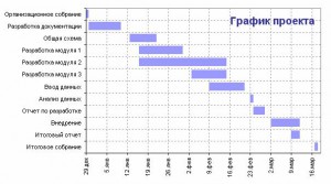
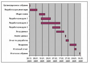
Current tasks will be interrupted by a line, and if the full side is on the left of the line, it means they are late in scheduling, and if the full side is on the right of the line, it means they are ahead of schedule. The right lines remain aloof from future tasks. Figure 1 shows that if today was October 15, activity 3 will be included in the planning, activities 4 and 5 will be delayed, and activity 7 will be ahead of the planning.
When you make a Gantt chart, just enter a reasonable number of tasks so that the chart fits on one page. For a more complex project, you can create sub-diagrams with detailed description deadlines for all subtasks that make up the main task.
![]()
If your table is created by analogy with the one presented above, then everything will work out for you, and we can continue to tell you how to build a Gantt chart in Excel.
Step #1: Building a Stacked Bar Chart
However, before you build a Gantt chart in Excel, you need to create another one - a bar chart. To do this, follow these steps:
In addition, it is very beneficial for the project team to have a task also be responsible for completing that task. Many times there are events in the context that are not a task, but you would like to highlight them in the Gantt chart. In the example above, renting a particular room is a very important point for further tasks, since this place must be explicitly mentioned in the press release. These moments represent "terminals" and are usually represented on the diagram as triangles with the tip pointing up.
How to draw a Gantt chart? To start, list all the tasks, the dates scheduled for their start and end, and who is responsible on a piece of paper. Also indicate the most important characteristics, as well as their details. If you have more than 15 or 20 tasks, you can divide the project into main tasks and subtasks, and then create a Gantt chart for the main tasks and another subtask chart for each of them.
- Highlight your table. To do this, move the cursor in one of its corners and, holding left button mouse (LMB), drag to another corner located diagonally.
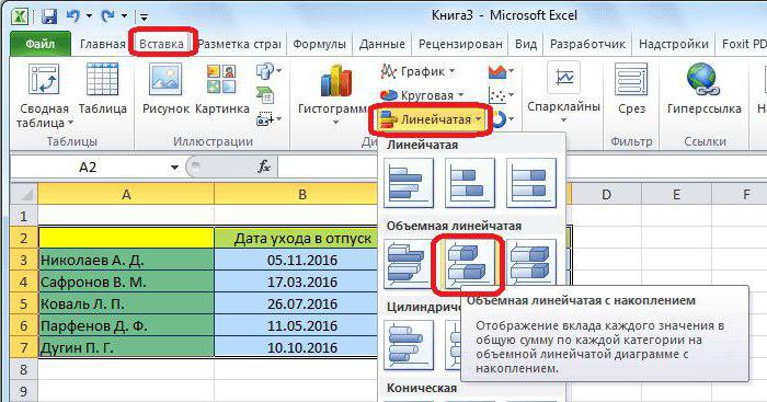
- Go to the "Insert" tab.
- Click on the "Bar" button, which is located in the "Charts" tool group.
- In the dropdown menu, click on any stacked chart. In this case it is "3D Stacked Bar".
The next step is to choose the unit of time you will use. If the project is less than three months, it is recommended to use days and longer projects to use weeks or months. For very short projects, you can even use the clock.
When you need to create a document yourself, you have three options. Use sequential options drawn on paper sheets with colored or colored pencils. While this solution is the most convenient, it will cause more problems with very frequent reviews.
Once you have done this, a corresponding diagram will appear on the program sheet. This means that the first stage is completed.
Step #2: Chart Formatting
At this stage of building a Gantt chart, in Excel it is necessary to make the first row invisible, which in our case is indicated in blue, that is, it is necessary that only the vacation period highlighted in red be on the chart. To do this, you need:
The advantage of this solution is that it allows you to update and correct the data frequently. Sequential charts are also easy to print. From the Page Setup option, select the horizontal orientation and center the chart vertically and horizontally. If the text is very small, you can print out the digraph on two pages and then assemble them together.
Another solution might be to increase the time unit or leave some less important tasks. Arrange the cells according to the chart elements you want. Enter the required information. To make gray bars representing the expected length of a task, select the cells and then use the Format Cells option.
- Click LMB on any blue area.
- Call the context menu by pressing RMB.
- In it, select the "Data Formatting" item.
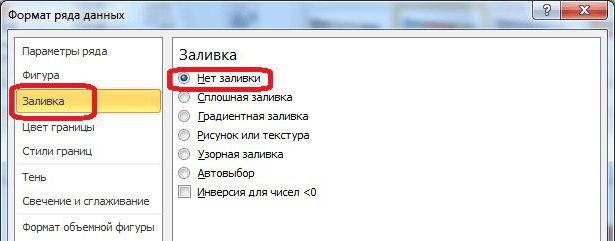
- Go to the Fill category.
- Select "No fill".
- Press the "Close" button.
Now, as you can see, the blue bars have disappeared from the diagram, of course, it would be more accurate to say that they have become invisible. This completes the second stage.
As the project progresses, change the fill color of the cells, from gray to black, to represent the percentage at which the pregnancy was completed. You know what your project is, make sure everyone else does too. Enter the name you want to give the chart. If you want to format text, you can do so from the main menu just like you would format any other text on the sheet.
Repeat for any other taskbar you want to change. 
Projects come in all shapes and sizes. If your project requires more than 25 lines in the template, it's simple and straightforward to add additional lines. Then a line will be added that has the appropriate formula to calculate task duration and the same formatting as other taskbars.
Step 3: Changing the Axis Format
The display of the axes does not currently match the correct pattern, so it needs to be changed. To do this, do the following:
- Click LMB on the names of employees to select them.
- Press RMB.
- In the menu that appears, click on "Format Axis".
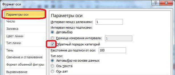
- A window will appear. In it, you need to go to the "Axis Options" category (usually it opens by default).
- In the category, you need to check the box next to "Reverse category order".
- Click Close.

To print only the Gantt chart, you first need to set the print area. 
Depending on the size of your chart, you will likely either need to adjust the scale of the chart to fit on one page, or lay out the chart across multiple pages and then manually copy them together to make one large printout.
Now the chart has changed its appearance - the dates are on top, and the names are turned upside down. So, firstly, it will be easier to perceive information, and secondly, it will be correct, so to speak, as required by GOST.
By the way, at this stage it would be nice to remove the legend in the chart, since it is not needed in this case. To do this, you need to initially select it by pressing the LMB and then pressing the DELETE key. Or you can delete it through the context menu called by RMB.

Again, depending on the size of your chart, you will likely need to either adjust the chart scale to one page, or map multiple pages and then manually copy them together to make one large printout. Project management is one of my favorite topics.
Project Dashboards and Project Management
The Gantt chart is the traditional way to prepare and track a project plan. It shows activities on the left and dates on the top. The intersection of an activity cell and a date is highlighted if the activity is due on that date. Reporting is one of the most important aspects of project management.
The third step of the instruction on how to build a Gantt chart is completed, but this is far from the end, so we proceed directly to the next step.
Stage 4: changing the period
If you pay attention to the time period in the chart, you will notice that its values go beyond their boundaries, which, at least, looks ugly. Now we are going to fix this nuance.
- How is the project going?
- What are the important issues we should be concerned about?
- We track budget, resources, etc.
Project Dashboard Example
Scheduling and project management tools
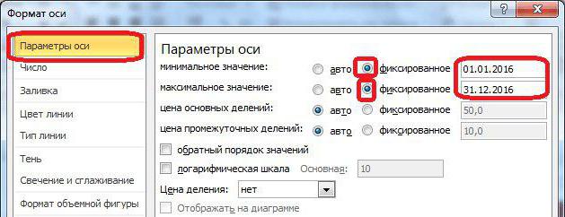
One of my bosses used to say, "If you can't measure, you can't handle." A good project manager always stays on top of the various things going on in the project. And this is where the image is tracked. On any given day, the project manager discovers tracking.First you need to select the time period itself. Then click the right mouse button on it and select the already familiar "Format Axis" item from the menu. In the window that appears, you need to be in the "Axis Options" category. There are two values \u200b\u200b"minimum" and "maximum", which you will need to change, but before starting, move the switch to the "Fixed" position. After that, enter the length of time that you need. By the way, in this window you can set the price of intermediate divisions if necessary.
Closed Questions - Sample Project Management Diagram
Problems in the project Risks in the project About the movement Activities in the project Make elements of different team members Schedules and budget and money. Graphs or visualizations help project managers understand where the project is. Closed questions: clearly indicate how well the problems in the project are being solved and indicate a trend. Budget vs Actual Charts: Show how the scope of the project, plans, costs are progressing against planned budgets. Just follow these links to get Project Management Templates and Tutorials.
After completing all the steps, click the "Close" button.
Stage number 5: entering the name
The last, fifth stage remains, which will complete the final formatting of our Gantt chart in Excel. In it we will set the name of the chart. Let's jump right into the process:
- Go to the "Layout" tab in the "Chart Tools" tab group. note that this group appears only when the chart is selected.
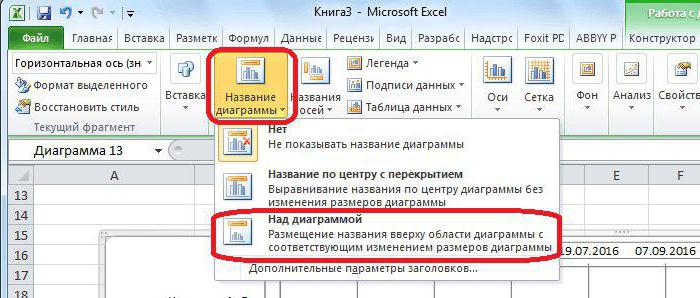
- In the "Layout" tab, you need to click on the "Chart Name" button, and in the drop-down list select the "Above the chart" item.
- In the field that appears in the diagram, you need to enter the name itself directly. It is advisable to choose one that fits the meaning.
We hope that our Excel Gantt chart example helped you, as this is the end of the creation. Of course, you can continue formatting further, but this will already affect, so to speak, the cosmetic part. By the way, if you do not want to bother and create it yourself, then you can find a bunch of Gantt chart templates in Excel on the Internet.
To begin with, we fill out a table listing the stages of the project, the start and end dates and the duration of each stage:
The task is to build standard means chart-calendar graph, as in the picture:
Let's go, step by step:
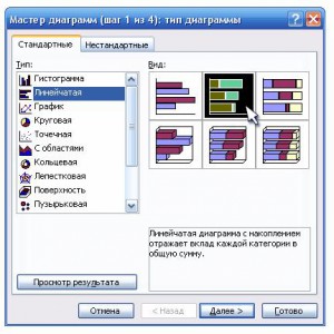
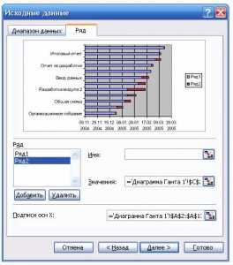
Let's select the source data for the chart - the range A2:B13 and select Insert - Chart from the menu, type - Stacked Bar:
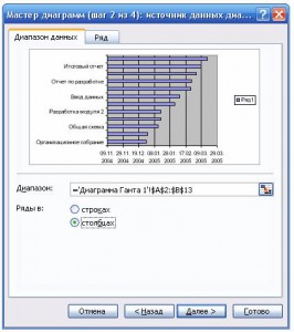
On the Series tab, click the Add button, place the cursor in the Values field and select cells with stage durations (C2:C13):
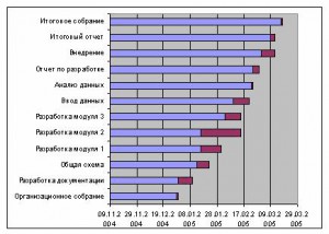
Do not be afraid - everything is going according to plan - you just need to "bring to mind" our diagram. To do this, click right click mouse on the vertical axis with the names of the stages and select in context menu Axis Format:
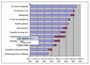
On the Scale tab in the window that opens, put two "checkmarks" - Reverse order of categories and Intersection with the Y axis in the maximum category. Click OK. Now let's get rid of the blue columns. Double-click on any of them and in the window that opens, select an invisible frame and a transparent fill. You should get the following:
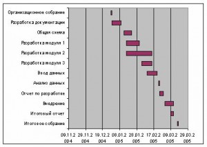
Looks like the truth already, right? It remains to correctly configure the range of data displayed on the chart. To do this, you need to find out the real contents of the cells from which the timeline begins and ends (yellow and green cells in the table). The fact is that Excel only displays the date in the cell as day-month-year, but actually stores any date in the cell as the number of days that have passed from 1.1.1900 to the current date. Select the yellow and green cells and, one by one, try to set the General Format for them (menu Format - Cells). It turns out 38350 and 38427, respectively. Let's add three more days to the end date - we get 38340. Remember these numbers.
It remains to right-click on the horizontal time axis and select Format Axis and enter these numbers in the Scale tab:
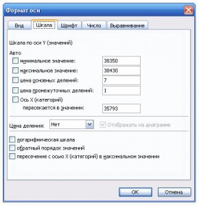
After clicking OK, the diagram will take the required form:
For convenience, you can download an example