This tutorial covers the basics of working with charts in Excel and is detailed guide by their construction. You will also learn how to combine two chart types, save a chart as a template, change the default chart type, resize or move a chart.

Excel charts are essential for visualizing data and keeping track of current trends. Microsoft Excel provides powerful functionality for working with charts, but finding the right tool can be difficult. Without a clear understanding of what types of charts are and for what purpose they are intended, you can spend a lot of time fiddling with various elements of the chart, and the result will only have a remote resemblance to what was intended.

We will start with the basics of creating charts and step by step how to create a chart in Excel. And even if you are new to this business, you can create your first chart in a few minutes and make it exactly as you need it.

Excel Charts - Basic Concepts

A chart (or graph) is a graphical representation of numerical data, where information is represented by symbols (bars, columns, lines, sectors, and so on). Graphs in Excel are usually created to make it easier to comprehend large amounts of information or to show the relationship between different subsets of data.

Microsoft Excel allows you to create many different types of charts: bar chart, column chart, line chart, pie and bubble chart, scatter and stock chart, donut and radar chart, area chart and surface chart.

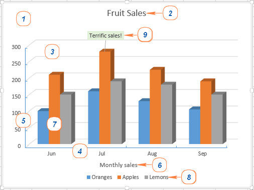
AT Excel charts there are many elements. Some of them are displayed by default, others, if necessary, can be added and configured manually.

Create a chart in Excel

To create a chart in Excel, start by entering numeric data into a worksheet and then follow these steps:

1. Prepare data for charting

Most Excel charts (such as bar charts or bar charts) do not require any special arrangement of data. The data can be in rows or columns, and Microsoft Excel will automatically suggest the most appropriate chart type (you can change it later).

To make a beautiful chart in Excel, the following points can be helpful:

• The chart legend uses either the column headings or data from the first column. Excel automatically selects the data for the legend based on the location of the source data.
• The data in the first column (or column headings) is used as the x-axis labels in the chart.
• The numeric data in the other columns is used to create the y-axis labels.

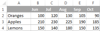
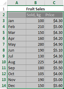
For example, let's build a graph based on the following table.

2. Choose what data to show on the chart

Select all the data you want to include in the Excel chart. Select the column headings you want to appear in the chart legend or as axis labels.

• If you need to build a graph based on adjacent cells, then just select one cell, and Excel will automatically add all adjacent cells containing data to the selection.
• To plot data in nonadjacent cells, select the first cell or range of cells, then press and hold ctrl, select the rest of the cells or ranges. Note that you can plot a non-contiguous cell or range graph only if the selected area forms a rectangle.

Advice: To select all used cells on a sheet, place the cursor in the first cell of the used area (click ctrl+home to move to a cell A1), then press Ctrl+Shift+End to expand the selection to the last used cell (lower right corner of the range).

3. Paste the chart into an Excel sheet

To add a chart to the current sheet, go to the tab Insert(Insert) section Diagrams(Charts) and click on the icon of the desired chart type.

In Excel 2013 and Excel 2016, you can click Recommended charts(Recommended Charts) to view a gallery of pre-made charts that best fit the selected data.

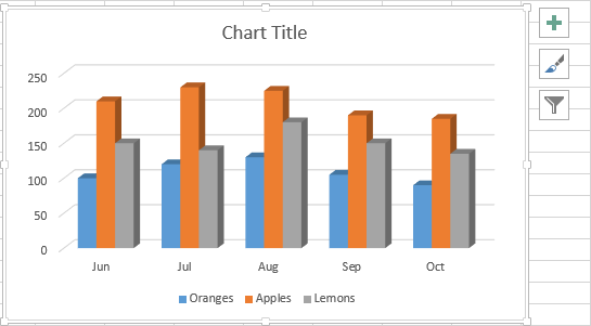
In this example, we are creating a 3D histogram. To do this, click on the arrow next to the histogram icon and select one of the chart subtypes in the category Volume histogram(3D Column).

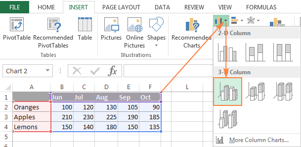
To select other chart types, click the link Other histograms(More Column Charts). A dialog box will open Insert a chart(Insert Chart) with a list of available histogram subtypes in the upper part of the window. At the top of the window, you can select other chart types available in Excel.

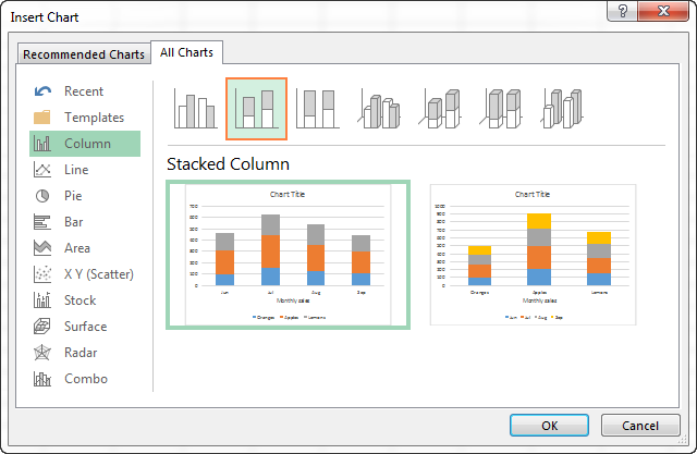
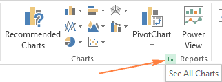
Advice: To see all available chart types immediately, click the button View all diagrams Diagrams(Charts) tab Insert(Insert) Menu ribbons.

In general, everything is ready. The chart is inserted on the current worksheet. Here is a voluminous histogram we got:

The graph looks good already, but there are still a few tweaks and improvements that can be made, as described in the section.

Create a combo chart in Excel to combine two types of charts

If you want to compare different types of data in an Excel chart, then you need to create a combo chart. For example, you can combine a bar or surface chart with a line chart to display data with very different dimensions, such as total revenue and units sold.

In Microsoft Excel 2010 and earlier, creating combo charts was a time consuming task. Excel 2013 and Excel 2016 solve this problem in four easy steps.

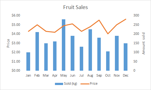
Finally, some touches can be added, such as the chart title and axis titles. The finished combo chart might look something like this:

Setting up Excel charts

As you have already seen, creating a chart in Excel is not difficult. But after adding a chart, you can change some of the standard elements to make the chart easier to read.

In the most latest versions Microsoft Excel 2013 and Excel 2016 have significantly improved charting and added a new way to access chart formatting options.

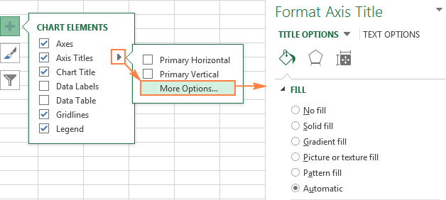
In general, there are 3 ways to customize charts in Excel 2016 and Excel 2013:

Click the icon to access additional options. Chart elements(Chart Elements), find the element you want to add or change in the list, and click the arrow next to it. The chart settings panel will appear to the right of the worksheet, here you can select the options you need:

We hope that this brief overview of chart customization features has helped you get a general idea of ​​how you can customize charts in Excel. In the following articles, we'll take a detailed look at how to customize various chart elements, including:

• How to move, adjust or hide the chart legend

Save a Chart Template in Excel

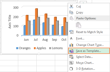
If you really like the created chart, then you can save it as a template ( .crtx file) and then apply this template to create other charts in Excel.

How to create a chart template

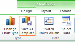
In Excel 2010 and earlier, the function Save as template(Save as Template) is located on the Menu Ribbon on the tab Constructor(Design) in the section Type of(type).

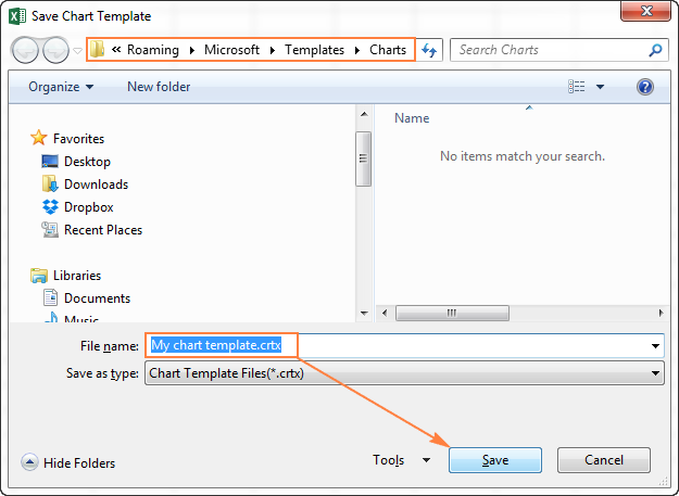
By default, the newly created chart template is saved to a special folder charts. All chart templates are automatically added to the section Templates(Templates), which appears in dialog boxes Insert a chart(Insert Chart) and Change the chart type(Change Chart Type) in Excel.

Please note that only those templates that have been saved in the folder charts will be available in Templates(Templates). Make sure you don't change the default folder when you save the template.

Advice: If you have downloaded chart templates from the Internet and want them to be available in Excel when you create a graph, save the downloaded template as .crtx file in folder charts:

C:\Users\Username\AppData\Roaming\Microsoft\Templates\Charts
C:\Users\UserName\AppData\Roaming\Microsoft\Templates\Charts

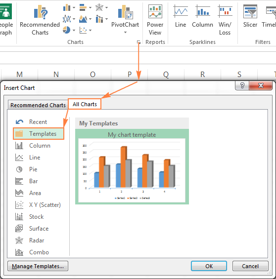
How to use the chart template

To create a chart in Excel from a template, open the dialog box Insert a chart(Insert Chart) by clicking on the button View all diagrams(See All Charts) in the lower right corner of the section Diagrams(Charts). On the tab All charts(All Charts) go to section Templates(Templates) and select the one you need from the available templates.

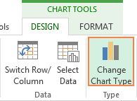
To apply a chart template to an already created chart, click right click mouse over the diagram and in the context menu select Change chart type(Change Chart Type). Or go to tab Constructor(Design) and press the button Change chart type(Change Chart Type) in the section Type of(type).

In both cases, a dialog box will open. Change the chart type(Change Chart Type), where in the section Templates(Templates) you can select the desired template.

How to delete a chart template in Excel

To delete a chart template, open the dialog box Insert a chart(Insert Chart), go to section Templates(Templates) and click the button Template Management(Manage Templates) in the lower left corner.

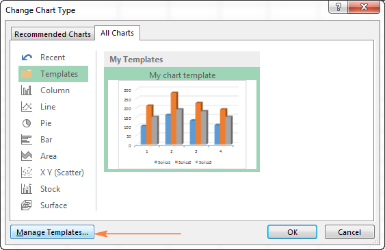
Button press Template Management(Manage Templates) will open the folder charts, which contains all existing templates. Right click on the template you want to delete and select Delete(Delete) in the context menu.

Using the default chart in Excel

The default Excel charts save a lot of time. Whenever you need to quickly create a chart or just look at trends in your data, you can create a chart in Excel with just one click! Simply select the data to be included in the chart and press one of the following keyboard shortcuts:

• Alt+F1 to insert a default chart on the current sheet.
• F11 to create a default chart on a new sheet.

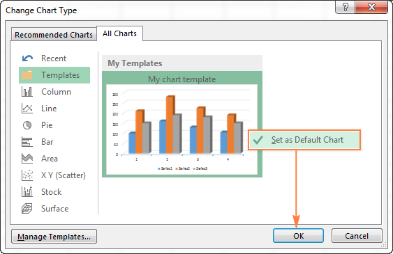
How to change the default chart type in Excel

When you create a chart in Excel, the bar chart is used as the default chart. To change the default chart format, do the following:

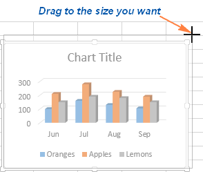
Resizing a Chart in Excel

To resize Excel charts, click on it and use the handles on the edges of the diagram to drag its borders.

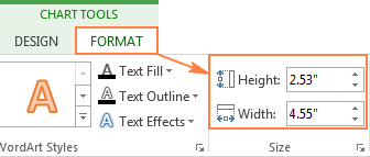
Another way is to enter the desired value in the fields Figure height(Shape Height) and Shape Width(Shape Width) in the section Size(Size) tab Format(Format).

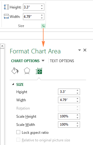
To access additional options, press the button View all diagrams(See All Charts) in the lower right corner of the section Diagrams(Charts).

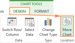
Move a chart in Excel

When creating a graph in Excel, it is automatically placed on the same sheet as the original data. You can move the chart anywhere on the sheet by dragging it with the mouse.

If you find it easier to work with the graph on a separate sheet, you can move it there as follows:

If you want to move the chart to an existing sheet, select the option on existing sheet(Object in) and select the desired sheet from the drop-down list.

To export a chart outside of Excel, right-click on the chart border and click Copy(Copy). Then open another program or application and paste the chart there. You can find some more ways to export charts in this article - .

This is how charts are created in Excel. I hope this overview of the main features of charts has been helpful. In the next lesson, we will go into detail about customizing various chart elements, such as chart title, axis titles, data labels, and so on. Thank you for your attention!

MS Excel has a built-in chart wizard that allows you not only to build charts and graphs of various types, but also to perform smoothing of experimental results.

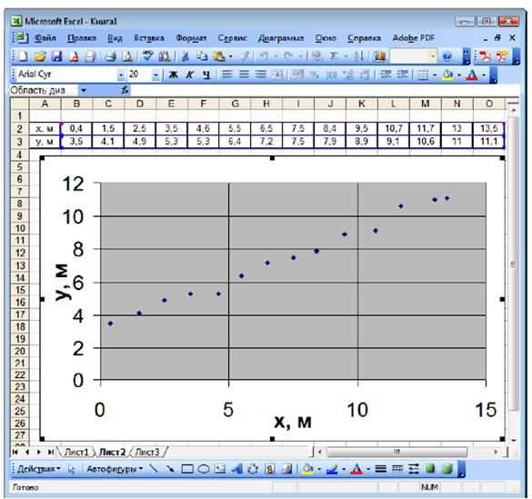
Consider the construction of a graph using MS Excel using the example of the dependence of body coordinates during rectilinear motion on the plane y=f(x). Let the experiment measure the coordinates of the body x and at at various points in time t. The measurement results are shown in the following table.

X, m	0,4	1,5	2,5	3,5	4,6	5,5	6,5	7,5	8,4	9,5	10,7	11,7		13,5
y, m	3,5	4,1	4,9	5,3	5,3	6,4	7,2	7,5	7,9	9,9	9,1	10,6		11,1

This example uses the same data as described for the least squares method and the graphical method.

Let's put this data in the second and third rows of the spreadsheet (Fig. 6). Select (using the mouse or keyboard) the cells in which the values ​​are located: AT 2, C2, ... O2, AT 3, C3, ... O3 (V2:03).

Above the table are several toolbars. One of them has a button. "Chart Master"(Fig. 6).

After pressing the button "Chart Master" a window will appear "Chart Wizard: Chart Type"(Fig. 7, a), in which we select the type of chart "Point" as it shown on the picture. This type of chart allows you to plot different data on both axes. Type of "Schedule" allows you to set values ​​only along the vertical axis, so it is rarely suitable for displaying the results of an experiment. For each type of chart, there are several types. In our example, the view will be used (Fig. 7, a), in which the points of the graph are not connected to each other. Let's press the button "Further".

A window will appear "Chart Wizard: Chart Data Source"(Fig. 7b). In this window, on the tab "Row" you can control which rows and columns will be used to plot data. Since before calling the chart wizard, we selected the area of ​​the table where the data necessary for plotting the chart are located, then in the field "Range" the numbers of the cells we have selected are automatically indicated, and a preview of the future diagram is shown at the top of the window. If the data is not displayed correctly, you can go to the tab "Row" and adjust the location of the data. In our case, the data is displayed correctly, so press the button "Further".

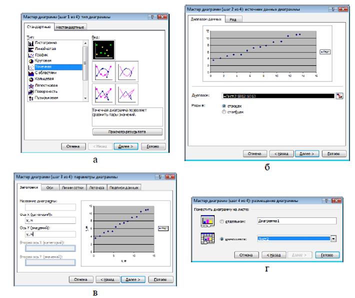
A new window will appear - "Chart Wizard: Chart Options"(Fig. 7, c). Here you can set labels for the axes and the entire chart, adjust the location of the legend, grid lines, etc.

Let's choose the following values:

On the tab "Headlines" in field "X-Axis" enter "x, m", and in the field "Y-Axis"- "mind".

On the tab "Grid Lines" in the proposed fields, place the “checkmarks” so that the main grid lines are displayed in the diagram field both along the X axis and along the Y axis.

On the "Legend" tab, uncheck the box "Add Legend", because we are going to display only one experimental dependence on the chart, so it makes no sense to label it. Let's press the button "Further".

will appear last window diagram wizard (Fig. 7, d), in which you can adjust the location of the diagram in spreadsheet. Agree with the proposed location and press the button "Ready".

A chart will appear in the spreadsheet (Figure 8), which (usually) still needs some tweaking.

Consider typical additional settings.

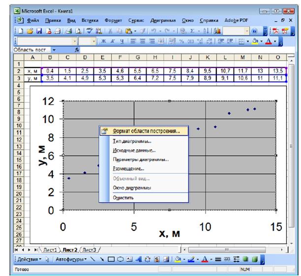
1. If the chart needs to be printed out, it is better to change the gray background of the chart to white. To do this, on the gray field (where there are no grid lines or dots), right-click to call context menu, in which we choose the item "Construction Area Format"(Fig. 9). A window will appear in which instead of a gray fill color, select white. In the same window, if necessary, you can set the color of the frame of the construction area.

2. The range of values ​​plotted along the axes on the chart by default is always wider than the data on which it is built. Change the scale of the horizontal axis. To do this, on one of the numbers signed along the horizontal axis, click the right mouse button to call the context menu, in which we select the item "Format Axis"(Fig. 10, a).

A window will appear "Format Axis"(Fig. 10, b).

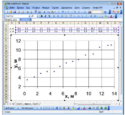Fig.10

On the tab "Scale" into the fields "Minimum value" and "Maximum Value" instead of the values ​​0 and 15, enter 0 and 14 respectively, and the value of the field "Price of the main divisions" set to 2. Press the button "OK".

Similarly, for the vertical axis, set the minimum value to 2. The maximum value is 12, and the price of the main divisions is 2.

The result is a graph as shown in Fig. eleven.

3. Construction of a smoothing curve. To do this, right-click on one of the graph points, in the context menu that appears, select the item "Add trend line"(Fig. 12, a).

A window will appear "Trend Line"(Fig. 12, b).

Here you can set the type and parameters of the smoothing curve. Six types of smoothing are available. In the experiment, the results of which are processed in this example, the rectilinear motion of a body on a plane was studied, so the dependence y = f (x) should be linear.

Therefore, we choose the type of trend line "Linear"(Fig. 12, b).

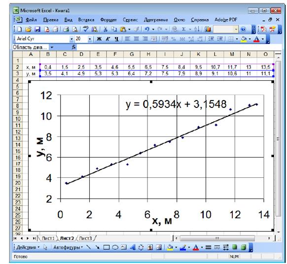
On the tab "Parameters"(Fig. 12, c) tick the box "Show Equation on Diagram" and press the button "OK".

Smoothing line coefficients (trend lines) are calculated using the least squares method.

We get a graph in the form shown in Fig. 13.

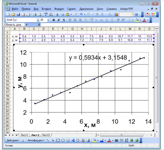MS Excel charts have a large number of customizable options. You can learn how to work with these parameters on your own, based on the principles described above.

OPTIONS FOR INDIVIDUAL TASKS FOR GRAPHIC REPRESENTATION OF RESEARCH RESULTS USING MS Excel

According to the experimental data available in task No. 2 at 1 , at 2 , at 3 ,…y n and X 1 , X 2 , X 3 ,…x p,, build a dependency graph at= f(x).