17.02.2017

Excel is a spreadsheet. It can be used to create a variety of reports. In this program, it is very convenient to perform various calculations. Many do not use even half of Excel's capabilities.

You may need to find the average value of numbers at school, as well as during work. The classic way determining the arithmetic mean without the use of programs is to add all the numbers, and then the resulting amount must be divided by the number of terms. If the numbers are large enough, or if the operation needs to be performed many times for reporting purposes, the calculations can take a long time. This is an irrational waste of time and effort, it is much better to use the capabilities of Excel.

Finding the arithmetic mean

Many data are already initially recorded in Excel, but if this does not happen, it is necessary to transfer the data to a table. Each number for the calculation must be in a separate cell.

Method 1: Calculate the average value through the "Function Wizard"

In this method, you need to write a formula for calculating the arithmetic mean and apply it to the specified cells.

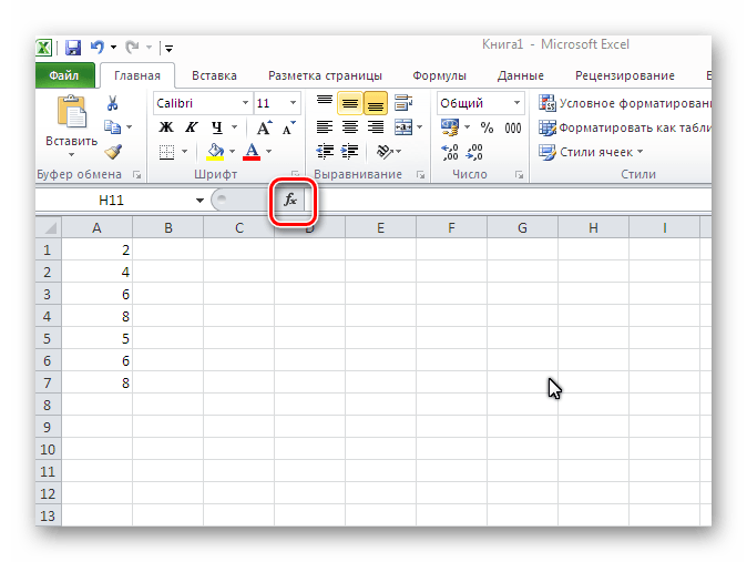
The main inconvenience of this method is that you have to manually enter cells for each term. In the presence of a large number numbers is not very convenient.

Method 2: Automatic calculation of the result in selected cells

In this method, the calculation of the arithmetic mean is carried out in just a couple of mouse clicks. Very handy for any number of numbers.

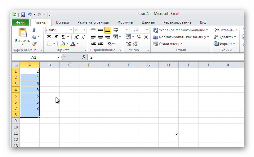
The disadvantage of this method is the calculation of the average value only for numbers located nearby. If the necessary terms are scattered, then they cannot be selected for calculation. It is not even possible to select two columns, in which case the results will be presented separately for each of them.

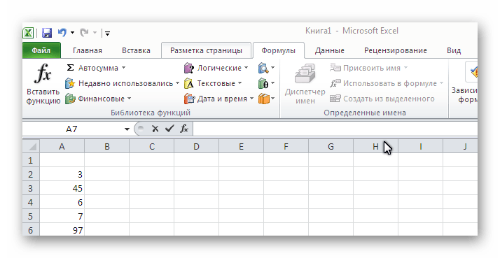
Method 3: Using the formula bar

Another way to go to the function window:

Most fast way, in which you do not need to search for items in the menu for a long time.

Method 4: Manual Entry

It is not necessary to use the tools in the Excel menu to calculate the average value, you can manually write the necessary function.

Fast and convenient way for those who prefer to create formulas with their own hands, rather than looking for ready-made programs in the menu.

Thanks to these features, it is very easy to calculate the average value of any numbers, regardless of their number, and you can also compile statistics without manually calculating them. With the help of the tools of the Excel program, any calculations are much easier to make than in the mind or using a calculator.

In order to find the average value in Excel (whether it is a numerical, textual, percentage or other value), there are many functions. And each of them has its own characteristics and advantages. After all, certain conditions can be set in this task.

For example, the average values ​​of a series of numbers in Excel are calculated using statistical functions. You can also manually enter your own formula. Let's consider various options.

How to find the arithmetic mean of numbers?

To find the arithmetic mean, you add all the numbers in the set and divide the sum by the number. For example, a student's grades in computer science: 3, 4, 3, 5, 5. What goes for a quarter: 4. We found the arithmetic mean using the formula: \u003d (3 + 4 + 3 + 5 + 5) / 5.

How to do it quickly using Excel functions? Take for example a series of random numbers in a string:

Or: make the cell active and simply manually enter the formula: =AVERAGE(A1:A8).

Now let's see what else the AVERAGE function can do.

Find the arithmetic mean of the first two and last three numbers. Formula: =AVERAGE(A1:B1;F1:H1). Result:

Average by condition

The condition for finding the arithmetic mean can be a numerical criterion or a text one. We will use the function: =AVERAGEIF().

Find the arithmetic mean of numbers that are greater than or equal to 10.

Function: =AVERAGEIF(A1:A8,">=10")

The result of using the AVERAGEIF function on the condition ">=10":

The third argument - "Averaging range" - is omitted. First, it is not required. Secondly, the range parsed by the program contains ONLY numeric values. In the cells specified in the first argument, the search will be performed according to the condition specified in the second argument.

Attention! The search criterion can be specified in a cell. And in the formula to make a reference to it.

Let's find the average value of the numbers by the text criterion. For example, the average sales of the product "tables".

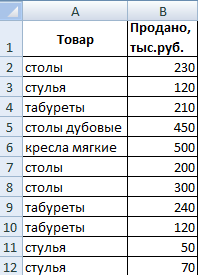
The function will look like this: =AVERAGEIF($A$2:$A$12;A7;$B$2:$B$12). Range - a column with product names. The search criterion is a link to a cell with the word "tables" (you can insert the word "tables" instead of the link A7). Averaging range - those cells from which data will be taken to calculate the average value.

As a result of calculating the function, we obtain the following value:

Attention! For a text criterion (condition), the averaging range must be specified.

How to calculate the weighted average price in Excel?

How do we know the weighted average price?

Formula: =SUMPRODUCT(C2:C12,B2:B12)/SUM(C2:C12).

Using the SUMPRODUCT formula, we find out the total revenue after the sale of the entire quantity of goods. And the SUM function - sums up the quantity of goods. By dividing the total revenue from the sale of goods by the total number of units of goods, we found the weighted average price. This indicator takes into account the "weight" of each price. Its share in the total mass of values.

Standard deviation: formula in Excel

Distinguish between the standard deviation for the general population and for the sample. In the first case, this is the root of the general variance. In the second, from the sample variance.

To calculate this statistical indicator, a dispersion formula is compiled. The root is taken from it. But in Excel there is a ready-made function for finding the standard deviation.

The standard deviation is linked to the scale of the source data. This is not enough for a figurative representation of the variation of the analyzed range. To get the relative level of scatter in the data, the coefficient of variation is calculated:

standard deviation / arithmetic mean

The formula in Excel looks like this:

STDEV (range of values) / AVERAGE (range of values).

The coefficient of variation is calculated as a percentage. Therefore, we set the percentage format in the cell.

For successful solution problem 19 from part 3 you need to know some Excel functions. One of these functions is AVERAGE. Let's consider it in more detail.

excel allows you to find the arithmetic mean of the arguments. The syntax for this function is:

AVERAGE(number1, [number2],…)

Do not forget that entering a formula into a cell begins with the "=" sign.

In parentheses, we can list the numbers whose average we want to find. For example, if we write in a cell =AVERAGE(1, 2, -7, 10, 7, 5, 9), then we get 3.857142857. This is easy to check - if we add all the numbers in brackets (1 + 2 + (-7) + 10 + 7 + 5 + 9 = 27) and divide by their number (7), we get 3.857142857142857.

Notice the numbers in parentheses separated by a semicolon (; ). Thus, we can specify up to 255 numbers.

For examples, I'm using Microsort Excel 2010.

In addition, with the help AVERAGE functions we can find average value of a range of cells. Suppose we have some numbers stored in the range A1:A7, and we want to find their arithmetic mean.

Let's put in cell B1 the arithmetic mean of the range A1:A7. To do this, place the cursor in cell B1 and write =AVERAGE(A1:A7). In parentheses, I indicated the range of cells. Note that the delimiter is the character colon (: ). It would be even easier to do - write in cell B1 =AVERAGE(, and then select the desired range with the mouse.

As a result, in cell B1 we will get the number 15.85714286 - this is the arithmetic mean of the range A1:A7.

As a warm-up, I propose to find the average value of numbers from 1 to 100 (1, 2, 3, etc. up to 100). The first person to answer correctly in the comments will receive 50 rubles to the phone We are working.

Instruction

Let there be a set of four numbers. Need to find average meaning this set. To do this, we first find the sum of all these numbers. Let's say these numbers are 1, 3, 8, 7. Their sum is S = 1 + 3 + 8 + 7 = 19. The set of numbers must consist of numbers of the same sign, otherwise the meaning of calculating the average value is lost.

Average meaning set of numbers is equal to the sum of the numbers S divided by the number of these numbers. That is, it turns out that average meaning equals: 19/4 = 4.75.

To set the number can also be found not only average arithmetic, but average geometric. The geometric mean of several positive real numbers is a number that can replace each of these numbers so that their product does not change. The geometric mean G is found by the formula: the root of the Nth degree of the product of a set of numbers, where N is the number of numbers in the set. Consider the same set of numbers: 1, 3, 8, 7. Find them average geometric. To do this, we calculate the product: 1 * 3 * 8 * 7 = 168. Now from the number 168 it is necessary to extract the root of the 4th degree: G = (168) ^ 1/4 = 3.61. Thus average the geometric set of numbers is 3.61.

Average the geometric mean is generally used less frequently than the arithmetic mean, but it can be useful when calculating the average of indicators that change over time (the salary of an individual employee, the dynamics of academic performance, etc.).

You will need

• Engineering Calculator

Instruction

In order to find the geometric mean of a series of numbers, you first need to multiply all these numbers. For example, you are given a set of five indicators: 12, 3, 6, 9 and 4. Let's multiply all these numbers: 12x3x6x9x4=7776.

Now, from the resulting number, you need to extract the root of the degree equal to the number of elements in the series. In our case, from the number 7776, you will need to extract the fifth degree root using an engineering calculator. The number obtained after this operation - in this case the number 6 - will be the geometric mean for the original group of numbers.

If you don’t have an engineering calculator at hand, then you can calculate the geometric mean of a series of numbers using the CPGEOM function in Excel or using one of the online calculators specifically designed to calculate geometric mean values.

note

If you need to find the geometric mean for just two numbers, then you will not need an engineering calculator: you can extract the second degree root (square root) of any number using the most common calculator.

Helpful advice

Unlike the arithmetic mean, the geometric mean is not so strongly influenced by large deviations and fluctuations between individual values ​​in the studied set of indicators.

Sources:

• Online calculator that calculates the geometric mean
• geometric mean formula

Average value is one of the characteristics of a set of numbers. Represents a number that cannot be outside the range defined by the largest and smallest values ​​in this set of numbers. Average arithmetic value - the most commonly used variety of averages.

Instruction

Add all the numbers in the set and divide them by the number of terms to get the arithmetic mean. Depending on the specific conditions of the calculation, it is sometimes easier to divide each of the numbers by the number of values ​​in the set and sum the result.

Use, for example, the calculator included with Windows if it is not possible to calculate the arithmetic mean in your head. You can open it using the program launcher dialog. To do this, press the "hot keys" WIN + R or click the "Start" button and select the "Run" command from the main menu. Then type calc into the input field and press Enter on the keyboard or click the OK button. The same can be done through the main menu - open it, go to the "All Programs" section and in the "Standard" section and select the "Calculator" line.

Enter all the numbers in the set in succession by pressing the Plus key on the keyboard after each of them (except the last one) or by clicking the corresponding button in the calculator interface. You can also enter numbers both from the keyboard and by clicking the corresponding interface buttons.

Press the slash key or click this icon in the calculator interface after entering the last value of the set and print the number of numbers in the sequence. Then press the equal sign and the calculator will calculate and display the arithmetic mean.

You can use a spreadsheet editor for the same purpose. Microsoft Excel. In this case, start the editor and enter all the values ​​of the sequence of numbers into adjacent cells. If after entering each number you press Enter or the down or right arrow key, the editor itself will move the input focus to the adjacent cell.

Select all the entered values ​​and in the lower left corner of the editor window (in the status bar) you will see the arithmetic mean for the selected cells.

Click the cell next to the last number you entered, if you don't want to just see the arithmetic mean. Expand the drop-down list with the image of the Greek letter sigma (Σ) in the Editing group of commands on the Home tab. Select the line " Average” and the editor will insert the desired formula for calculating the arithmetic mean in the selected cell. Press the Enter key and the value will be calculated.

The arithmetic mean is one of the measures of central tendency, widely used in mathematics and statistical calculations. Finding the arithmetic average of several values ​​​​is very simple, but each task has its own nuances, which are simply necessary to know in order to perform correct calculations.

What is the arithmetic mean

The arithmetic mean determines the average value for the entire original array of numbers. In other words, from a certain set of numbers, a value common to all elements is selected, the mathematical comparison of which with all elements is approximately equal. The arithmetic mean is used primarily in the preparation of financial and statistical reports or for calculating the quantitative results of such experiments.

How to find the arithmetic mean

The search for the arithmetic mean for an array of numbers should begin with determining the algebraic sum of these values. For example, if the array contains the numbers 23, 43, 10, 74 and 34, then their algebraic sum will be 184. When writing, the arithmetic mean is denoted by the letter μ (mu) or x (x with a bar). Next, the algebraic sum should be divided by the number of numbers in the array. In this example, there were five numbers, so the arithmetic mean will be 184/5 and will be 36.8.

Features of working with negative numbers

If there are negative numbers in the array, then the arithmetic mean is found using a similar algorithm. There is a difference only when calculating in the programming environment, or if there are additional conditions in the task. In these cases, finding the arithmetic mean of numbers with different signs comes down to three steps:

1. Finding the common arithmetic mean by the standard method;
2. Finding the arithmetic mean of negative numbers.
3. Calculation of the arithmetic mean of positive numbers.

The responses of each of the actions are written separated by commas.

Natural and decimal fractions

If the array of numbers is represented by decimal fractions, the solution occurs according to the method of calculating the arithmetic mean of integers, but the result is reduced according to the requirements of the problem for the accuracy of the answer.

When working with natural fractions, they should be reduced to a common denominator, which is multiplied by the number of numbers in the array. The numerator of the answer will be the sum of the given numerators of the original fractional elements.

The geometric mean of numbers depends not only on the absolute value of the numbers themselves, but also on their number. Do not confuse the geometric mean and the arithmetic mean of numbers, since they are found using different methods. The geometric mean is always less than or equal to the arithmetic mean.

To find the geometric mean of more than two numbers, also use the basic rule. To do this, find the product of all the numbers for which you want to find the geometric mean. From the resulting product, extract the root of the degree equal to the number of numbers. For example, to find the geometric mean of the numbers 2, 4, and 64, find their product. 2•4•64=512. Since you need to find the result of the geometric mean of three numbers, extract the root of the third degree from the product. It is difficult to do this verbally, so use an engineering calculator. To do this, it has a button "x ^ y". Dial the number 512, press the "x^y" button, then dial the number 3 and press the "1/x" button, to find the value 1/3, press the "=" button. We get the result of raising 512 to the power of 1/3, which corresponds to the root of the third degree. Get 512^1/3=8. This is the geometric mean of the numbers 2.4 and 64.

Using an engineering calculator, you can find the geometric mean in another way. Find the log button on your keyboard. After that, take the logarithm for each of the numbers, find their sum and divide it by the number of numbers. From the resulting number, take the antilogarithm. This will be the geometric mean of the numbers. For example, in order to find the geometric mean of the same numbers 2, 4 and 64, make a set of operations on the calculator. Type the number 2, then press the log button, press the "+" button, type the number 4 and press log and "+" again, type 64, press log and "=". The result will be a number equal to the sum of the decimal logarithms of the numbers 2, 4 and 64. Divide the resulting number by 3, since this is the number of numbers by which the geometric mean is sought. From the result, take the antilogarithm by toggling the register key and use the same log key. The result is the number 8, this is the desired geometric mean.

note

The mean cannot be greater than the largest number in the set and less than the smallest.

Helpful advice

In mathematical statistics, the average value of a quantity is called the mathematical expectation.

Sources:

• how to calculate average
• Find the arithmetic mean of all integers from 1 to 1000
• Finding the geometric mean

In most cases, the data is concentrated around some central point. Thus, to describe any data set, it is enough to indicate the average value. Consider successively three numerical characteristics that are used to estimate the mean value of the distribution: arithmetic mean, median and mode.

Average

The arithmetic mean (often referred to simply as the mean) is the most common estimate of the mean of a distribution. It is the result of dividing the sum of all observed numerical values ​​by their number. For a sample of numbers X 1, X 2, ..., Xn, the sample mean (denoted by the symbol ) equals \u003d (X 1 + X 2 + ... + Xn) / n, or

where is the sample mean, n- sample size, Xi – i-th element samples.

Download note in or format, examples in format

Consider calculating the arithmetic average of the five-year average annual returns of 15 very high-risk mutual funds (Figure 1).

Rice. 1. Average annual return on 15 very high-risk mutual funds

The sample mean is calculated as follows:

This is a good return, especially when compared to the 3-4% return that bank or credit union depositors received over the same time period. If you sort the return values, it is easy to see that eight funds have a return above, and seven - below the average. The arithmetic mean acts as a balance point, so that low-income funds balance out high-income funds. All elements of the sample are involved in the calculation of the average. None of the other estimators of the distribution mean have this property.

When to calculate the arithmetic mean. Since the arithmetic mean depends on all elements of the sample, the presence of extreme values ​​significantly affects the result. In such situations, the arithmetic mean can distort the meaning of the numerical data. Therefore, when describing a data set containing extreme values, it is necessary to indicate the median or the arithmetic mean and the median. For example, if the return of the RS Emerging Growth fund is removed from the sample, the sample average of the return of the 14 funds decreases by almost 1% to 5.19%.

Median

The median is the middle value of an ordered array of numbers. If the array does not contain repeating numbers, then half of its elements will be less than and half more than the median. If the sample contains extreme values, it is better to use the median rather than the arithmetic mean to estimate the mean. To calculate the median of a sample, it must first be sorted.

This formula is ambiguous. Its result depends on whether the number is even or odd. n:

• If the sample contains an odd number of items, the median is (n+1)/2-th element.
• If the sample contains an even number of elements, the median lies between the two middle elements of the sample and is equal to the arithmetic mean calculated over these two elements.

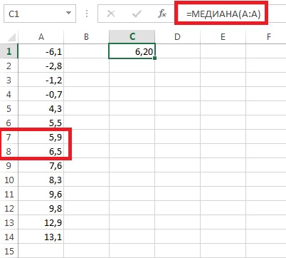
To calculate the median for a sample of 15 very high-risk mutual funds, we first need to sort the raw data (Figure 2). Then the median will be opposite the number of the middle element of the sample; in our example number 8. Excel has a special function =MEDIAN() that works with unordered arrays too.

Rice. 2. Median 15 funds

Thus, the median is 6.5. This means that half of the very high-risk funds do not exceed 6.5, while the other half do so. Note that the median of 6.5 is slightly larger than the median of 6.08.

If we remove the profitability of the RS Emerging Growth fund from the sample, then the median of the remaining 14 funds will decrease to 6.2%, that is, not as significantly as the arithmetic mean (Fig. 3).

Rice. 3. Median 14 funds

Fashion

The term was first introduced by Pearson in 1894. Fashion is the number that occurs most often in the sample (the most fashionable). Fashion describes well, for example, the typical reaction of drivers to a traffic signal to stop traffic. A classic example of the use of fashion is the choice of the size of the produced batch of shoes or the color of the wallpaper. If a distribution has multiple modes, then it is said to be multimodal or multimodal (has two or more "peaks"). The multimodality of distribution gives important information about the nature of the variable under study. For example, in sociological surveys, if a variable represents a preference or attitude towards something, then multimodality could mean that there are several distinctly different opinions. Multimodality is also an indicator that the sample is not homogeneous and that the observations may be generated by two or more "overlapped" distributions. Unlike the arithmetic mean, outliers do not affect the mode. For continuously distributed random variables, such as the average annual returns of mutual funds, the mode sometimes does not exist at all (or does not make sense). Since these indicators can take on a variety of values, repeating values ​​are extremely rare.

Quartiles

Quartiles are measures that are most commonly used to evaluate the distribution of data when describing the properties of large numerical samples. While the median splits the ordered array in half (50% of the array elements are less than the median and 50% are greater), quartiles break the ordered dataset into four parts. The Q 1 , median and Q 3 values ​​are the 25th, 50th and 75th percentile, respectively. The first quartile Q 1 is a number that divides the sample into two parts: 25% of the elements are less than, and 75% are more than the first quartile.

The third quartile Q 3 is a number that also divides the sample into two parts: 75% of the elements are less than, and 25% are more than the third quartile.

To calculate quartiles in versions of Excel prior to 2007, the function =QUARTILE(array, part) was used. Starting with Excel 2010, two functions apply:

• =QUARTILE.ON(array, part)
• =QUARTILE.EXC(array, part)

These two functions give slightly different values ​​(Figure 4). For example, when calculating the quartiles of a sample containing data on the average annual return of 15 very high-risk mutual funds, Q 1 = 1.8 or -0.7 for QUARTILE.INC and QUARTILE.EXC, respectively. By the way, the QUARTILE function used earlier corresponds to the modern QUARTILE.ON function. To calculate quartiles in Excel using the above formulas, the data array can be left unordered.

Rice. 4. Calculate quartiles in Excel

Let's emphasize again. Excel can calculate quartiles for univariate discrete series, containing the values ​​of a random variable. The calculation of quartiles for a frequency-based distribution is given in the section below.

geometric mean

Unlike the arithmetic mean, the geometric mean measures how much a variable has changed over time. The geometric mean is the root n th degree from the product n values ​​(in Excel, the function = CUGEOM is used):

G= (X 1 * X 2 * ... * X n) 1/n

A similar parameter - the geometric mean of the rate of return - is determined by the formula:

G \u003d [(1 + R 1) * (1 + R 2) * ... * (1 + R n)] 1 / n - 1,

where R i- rate of return i-th period of time.

For example, suppose the initial investment is $100,000. By the end of the first year, it drops to $50,000, and by the end of the second year, it recovers to the original $100,000. The rate of return on this investment over a two-year period is equal to 0, since the initial and final amount of funds are equal to each other. However, the arithmetic average of annual rates of return is = (-0.5 + 1) / 2 = 0.25 or 25%, since the rate of return in the first year R 1 = (50,000 - 100,000) / 100,000 = -0.5 , and in the second R 2 = (100,000 - 50,000) / 50,000 = 1. At the same time, the geometric mean of the rate of return for two years is: G = [(1–0.5) * (1 + 1 )] 1/2 – 1 = ½ – 1 = 1 – 1 = 0. Thus, the geometric mean more accurately reflects the change (more precisely, the absence of change) in the volume of investments over the biennium than the arithmetic mean.

Interesting Facts. First, the geometric mean will always be less than the arithmetic mean of the same numbers. Except for the case when all the taken numbers are equal to each other. Secondly, having considered the properties of a right triangle, one can understand why the mean is called geometric. The height of a right-angled triangle, lowered to the hypotenuse, is the average proportional between the projections of the legs on the hypotenuse, and each leg is the average proportional between the hypotenuse and its projection on the hypotenuse (Fig. 5). This gives a geometric way of constructing the geometric mean of two (lengths) segments: you need to build a circle on the sum of these two segments as a diameter, then the height, restored from the point of their connection to the intersection with the circle, will give the required value:

Rice. 5. The geometric nature of the geometric mean (figure from Wikipedia)

The second important property of numerical data is their variation characterizing the degree of dispersion of the data. Two different samples can differ both in mean values ​​and in variations. However, as shown in fig. 6 and 7, two samples can have the same variation but different means, or the same mean and completely different variation. The data corresponding to polygon B in Fig. 7 change much less than the data from which polygon A was built.

Rice. 6. Two symmetric bell-shaped distributions with the same spread and different mean values

Rice. 7. Two symmetric bell-shaped distributions with the same mean values ​​and different scatter

There are five estimates of data variation:

• span,
• interquartile range,
• dispersion,
• standard deviation,
• the coefficient of variation.

scope

The range is the difference between the largest and smallest elements of the sample:

Swipe = XMax-XMin

The range of a sample containing the average annual returns of 15 very high-risk mutual funds can be calculated using an ordered array (see Figure 4): range = 18.5 - (-6.1) = 24.6. This means that the difference between the highest and lowest average annual returns for very high risk funds is 24.6%.

The range measures the overall spread of the data. Although the sample range is a very simple estimate of the total spread of the data, its weakness is that it does not take into account exactly how the data is distributed between the minimum and maximum elements. This effect is well seen in Fig. 8 which illustrates samples having the same range. The B scale shows that if the sample contains at least one extreme value, the sample range is a very inaccurate estimate of the scatter of the data.

Rice. 8. Comparison of three samples with the same range; the triangle symbolizes the support of the balance, and its location corresponds to the average value of the sample

Interquartile range

The interquartile, or mean, range is the difference between the third and first quartiles of the sample:

Interquartile range \u003d Q 3 - Q 1

This value makes it possible to estimate the spread of 50% of the elements and not to take into account the influence of extreme elements. The interquartile range for a sample containing data on the average annual returns of 15 very high-risk mutual funds can be calculated using the data in Fig. 4 (for example, for the function QUARTILE.EXC): Interquartile range = 9.8 - (-0.7) = 10.5. The interval between 9.8 and -0.7 is often referred to as the middle half.

It should be noted that the Q 1 and Q 3 values, and hence the interquartile range, do not depend on the presence of outliers, since their calculation does not take into account any value that would be less than Q 1 or greater than Q 3 . The total quantitative characteristics, such as the median, the first and third quartiles, and the interquartile range, which are not affected by outliers, are called robust indicators.

While the range and interquartile range provide an estimate of the total and mean scatter of the sample, respectively, neither of these estimates takes into account exactly how the data are distributed. Variance and standard deviation free from this shortcoming. These indicators allow you to assess the degree of fluctuation of the data around the mean. Sample variance is an approximation of the arithmetic mean calculated from the squared differences between each sample element and the sample mean. For a sample of X 1 , X 2 , ... X n the sample variance (denoted by the symbol S 2 is given by the following formula:

In general, the sample variance is the sum of the squared differences between the sample elements and the sample mean, divided by a value equal to the sample size minus one:

where - arithmetic mean, n- sample size, X i - i-th sample element X. In Excel before version 2007, the function =VAR() was used to calculate the sample variance, since version 2010, the function =VAR.V() is used.

The most practical and widely accepted estimate of data scatter is standard deviation. This indicator is denoted by the symbol S and is equal to the square root of the sample variance:

In Excel before version 2007, the =STDEV() function was used to calculate the standard deviation, from version 2010 the =STDEV.V() function is used. To calculate these functions, the data array can be unordered.

Neither the sample variance nor the sample standard deviation can be negative. The only situation in which the indicators S 2 and S can be zero is if all elements of the sample are equal. In this completely improbable case, the range and interquartile range are also zero.

Numeric data is inherently volatile. Any variable can take on a set different values. For example, different mutual funds have different rates of return and loss. Due to the variability of numerical data, it is very important to study not only estimates of the mean, which are summative in nature, but also estimates of the variance, which characterize the scatter of the data.

The variance and standard deviation allow us to estimate the spread of data around the mean, in other words, to determine how many elements of the sample are less than the mean, and how many are greater. The dispersion has some valuable mathematical properties. However, its value is the square of a unit of measure - a square percentage, a square dollar, a square inch, etc. Therefore, a natural estimate of the variance is the standard deviation, which is expressed in the usual units of measurement - percent of income, dollars or inches.

The standard deviation allows you to estimate the amount of fluctuation of the sample elements around the mean value. In almost all situations, the majority of observed values ​​lie within plus or minus one standard deviation from the mean. Therefore, knowing the arithmetic mean of the sample elements and the standard sample deviation, it is possible to determine the interval to which the bulk of the data belongs.

The standard deviation of returns on 15 very high-risk mutual funds is 6.6 (Figure 9). This means that the profitability of the bulk of funds differs from the average value by no more than 6.6% (i.e., it fluctuates in the range from – S= 6.2 – 6.6 = –0.4 to +S= 12.8). In fact, this interval contains a five-year average annual return of 53.3% (8 out of 15) of funds.

Rice. 9. Standard deviation

Note that in the process of summing the squared differences, items that are farther from the mean gain more weight than items that are closer. This property is the main reason why the arithmetic mean is most often used to estimate the mean of a distribution.

The coefficient of variation

Unlike previous scatter estimates, the coefficient of variation is a relative estimate. It is always measured as a percentage, not in the original data units. The coefficient of variation, denoted by the symbols CV, measures the scatter of the data around the mean. The coefficient of variation is equal to the standard deviation divided by the arithmetic mean and multiplied by 100%:

where S- standard sample deviation, - sample mean.

The coefficient of variation allows you to compare two samples, the elements of which are expressed in different units of measurement. For example, the manager of a mail delivery service intends to upgrade the fleet of trucks. When loading packages, there are two types of restrictions to consider: the weight (in pounds) and the volume (in cubic feet) of each package. Assume that in a sample of 200 bags, the average weight is 26.0 pounds, the standard deviation of the weight is 3.9 pounds, the average package volume is 8.8 cubic feet, and the standard deviation of the volume is 2.2 cubic feet. How to compare the spread of weight and volume of packages?

Since the units of measurement for weight and volume differ from each other, the manager must compare the relative spread of these values. The weight variation coefficient is CV W = 3.9 / 26.0 * 100% = 15%, and the volume variation coefficient CV V = 2.2 / 8.8 * 100% = 25% . Thus, the relative scatter of packet volumes is much larger than the relative scatter of their weights.

Distribution form

The third important property of the sample is the form of its distribution. This distribution can be symmetrical or asymmetric. To describe the shape of a distribution, it is necessary to calculate its mean and median. If these two measures are the same, the variable is said to be symmetrically distributed. If the mean value of a variable is greater than the median, its distribution has a positive skewness (Fig. 10). If the median is greater than the mean, the distribution of the variable is negatively skewed. Positive skewness occurs when the mean increases to unusually high values. Negative skewness occurs when the mean decreases to unusually small values. A variable is symmetrically distributed if it does not take on any extreme values ​​in either direction, such that large and small values ​​of the variable cancel each other out.

Rice. 10. Three types of distributions

The data depicted on the A scale have a negative skewness. This figure shows a long tail and left skew caused by unusually small values. These extremely small values ​​shift the mean value to the left, and it becomes less than the median. The data shown on scale B are distributed symmetrically. The left and right halves of the distribution are their mirror images. Large and small values ​​balance each other, and the mean and median are equal. The data shown on scale B has a positive skewness. This figure shows a long tail and skew to the right, caused by the presence of unusually high values. These too large values ​​shift the mean to the right, and it becomes larger than the median.

In Excel, descriptive statistics can be obtained using the add-in Analysis package. Go through the menu Data → Data analysis, in the window that opens, select the line Descriptive statistics and click Ok. In the window Descriptive statistics be sure to indicate input interval(Fig. 11). If you want to see descriptive statistics on the same sheet as the original data, select the radio button output interval and specify the cell where you want to place the upper left corner of the displayed statistics (in our example, $C$1). If you want to output data to a new sheet or to a new workbook, simply select the appropriate radio button. Check the box next to Final statistics. Optionally, you can also choose Difficulty level,k-th smallest andk-th largest.

If on deposit Data in area Analysis you don't see the icon Data analysis, you must first install the add-on Analysis package(see, for example,).

Rice. 11. Descriptive statistics of the five-year average annual returns of funds with very high levels of risk, calculated using the add-on Data analysis Excel programs

Excel calculates a number of statistics discussed above: mean, median, mode, standard deviation, variance, range ( interval), minimum, maximum, and sample size ( check). In addition, Excel calculates some new statistics for us: standard error, kurtosis, and skewness. standard error equals the standard deviation divided by the square root of the sample size. asymmetry characterizes the deviation from the symmetry of the distribution and is a function that depends on the cube of differences between the elements of the sample and the mean value. Kurtosis is a measure of the relative concentration of data around the mean versus the tails of the distribution, and depends on the differences between the sample and the mean raised to the fourth power.

Calculation of descriptive statistics for the general population

The mean, scatter, and shape of the distribution discussed above are sample-based characteristics. However, if the dataset contains numerical measurements of the entire population, then its parameters can be calculated. These parameters include the mean, variance, and standard deviation of the population.

Expected value is equal to the sum of all values ​​of the general population divided by the volume of the general population:

where µ - expected value, Xi- i-th variable observation X, N- the volume of the general population. In Excel, to calculate the mathematical expectation, the same function is used as for the arithmetic mean: =AVERAGE().

Population variance equal to the sum of the squared differences between the elements of the general population and mat. expectation divided by the size of the population:

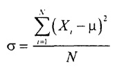
where σ2 is the variance of the general population. Excel prior to version 2007 uses the =VAR() function to calculate the population variance, starting with version 2010 =VAR.G().

population standard deviation is equal to the square root of the population variance:

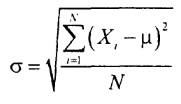
Excel prior to version 2007 uses =STDEV() to calculate the population standard deviation, starting with version 2010 =STDEV.Y(). Note that the formulas for population variance and standard deviation are different from the formulas for sample variance and standard deviation. When calculating sample statistics S2 and S the denominator of the fraction is n - 1, and when calculating the parameters σ2 and σ - the volume of the general population N.

rule of thumb

In most situations, a large proportion of observations are concentrated around the median, forming a cluster. In data sets with positive skewness, this cluster is located to the left (i.e., below) the mathematical expectation, and in sets with negative skewness, this cluster is located to the right (i.e., above) of the mathematical expectation. Symmetric data have the same mean and median, and the observations cluster around the mean, forming a bell-shaped distribution. If the distribution does not have a pronounced skewness, and the data is concentrated around a certain center of gravity, a rule of thumb can be used to estimate variability, which says: if the data has a bell-shaped distribution, then approximately 68% of the observations are less than one standard deviation from the mathematical expectation, Approximately 95% of the observations are within two standard deviations of the expected value, and 99.7% of the observations are within three standard deviations of the expected value.

Thus, the standard deviation, which is an estimate of the average fluctuation around the mathematical expectation, helps to understand how the observations are distributed and to identify outliers. It follows from the rule of thumb that for bell-shaped distributions, only one value in twenty differs from the mathematical expectation by more than two standard deviations. Therefore, values ​​outside the interval µ ± 2σ, can be considered outliers. In addition, only three out of 1000 observations differ from the mathematical expectation by more than three standard deviations. Thus, values ​​outside the interval µ ± 3σ are almost always outliers. For distributions that are highly skewed or not bell-shaped, the Biename-Chebyshev rule of thumb can be applied.

More than a hundred years ago, the mathematicians Bienamay and Chebyshev independently discovered a useful property of the standard deviation. They found that for any data set, regardless of the shape of the distribution, the percentage of observations that lie at a distance not exceeding k standard deviations from mathematical expectation, not less (1 – 1/ 2)*100%.

For example, if k= 2, the Biename-Chebyshev rule states that at least (1 - (1/2) 2) x 100% = 75% of the observations must lie in the interval µ ± 2σ. This rule is true for any k exceeding one. The Biename-Chebyshev rule is of a very general nature and is valid for distributions of any kind. It indicates the minimum number of observations, the distance from which to the mathematical expectation does not exceed a given value. However, if the distribution is bell-shaped, the rule of thumb more accurately estimates the concentration of data around the mean.

Computing descriptive statistics for a frequency-based distribution

If the original data is not available, the frequency distribution becomes the only source of information. In such situations, you can calculate the approximate values ​​of quantitative indicators of the distribution, such as the arithmetic mean, standard deviation, quartiles.

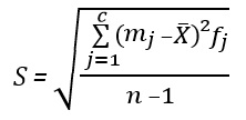
If the sample data is presented as a frequency distribution, an approximate value of the arithmetic mean can be calculated, assuming that all values ​​within each class are concentrated at the midpoint of the class:

where - sample mean, n- number of observations, or sample size, with- the number of classes in the frequency distribution, mj- middle point j-th class, fj- frequency corresponding to j-th class.

To calculate the standard deviation from the frequency distribution, it is also assumed that all values ​​within each class are concentrated at the midpoint of the class.

To understand how the quartiles of the series are determined based on frequencies, let us consider the calculation of the lower quartile based on the data for 2013 on the distribution of the Russian population by average per capita cash income (Fig. 12).

Rice. 12. The share of the population of Russia with per capita monetary income on average per month, rubles

To calculate the first quartile of the interval variation series, you can use the formula:

where Q1 is the value of the first quartile, xQ1 is the lower limit of the interval containing the first quartile (the interval is determined by the accumulated frequency, the first exceeding 25%); i is the value of the interval; Σf is the sum of the frequencies of the entire sample; probably always equal to 100%; SQ1–1 is the cumulative frequency of the interval preceding the interval containing the lower quartile; fQ1 is the frequency of the interval containing the lower quartile. The formula for the third quartile differs in that in all places, instead of Q1, you need to use Q3, and substitute ¾ instead of ¼.

In our example (Fig. 12), the lower quartile is in the range 7000.1 - 10,000, the cumulative frequency of which is 26.4%. The lower limit of this interval is 7000 rubles, the value of the interval is 3000 rubles, the accumulated frequency of the interval preceding the interval containing the lower quartile is 13.4%, the frequency of the interval containing the lower quartile is 13.0%. Thus: Q1 \u003d 7000 + 3000 * (¼ * 100 - 13.4) / 13 \u003d 9677 rubles.

Pitfalls associated with descriptive statistics

In this note, we looked at how to describe a dataset using various statistics that estimate its mean, scatter, and distribution. The next step is to analyze and interpret the data. So far, we have studied the objective properties of data, and now we turn to their subjective interpretation. Two mistakes lie in wait for the researcher: an incorrectly chosen subject of analysis and an incorrect interpretation of the results.

An analysis of the performance of 15 very high-risk mutual funds is fairly unbiased. He led to completely objective conclusions: all mutual funds have different returns, the spread of fund returns ranges from -6.1 to 18.5, and the average return is 6.08. The objectivity of data analysis is ensured by the correct choice of total quantitative indicators of the distribution. Several methods for estimating the mean and scatter of data were considered, and their advantages and disadvantages were indicated. How to choose the right statistics that provide an objective and unbiased analysis? If the data distribution is slightly skewed, should the median be chosen over the arithmetic mean? Which indicator more accurately characterizes the spread of data: standard deviation or range? Should the positive skewness of the distribution be indicated?

On the other hand, data interpretation is a subjective process. Different people come to different conclusions, interpreting the same results. Everyone has their own point of view. Someone considers the total average annual returns of 15 funds with a very high level of risk to be good and is quite satisfied with the income received. Others may think that these funds have too low returns. Thus, subjectivity should be compensated by honesty, neutrality and clarity of conclusions.

Ethical Issues

Data analysis is inextricably linked to ethical issues. One should be critical of the information disseminated by newspapers, radio, television and the Internet. Over time, you will learn to be skeptical not only about the results, but also about the goals, subject and objectivity of research. The famous British politician Benjamin Disraeli said it best: “There are three kinds of lies: lies, damned lies and statistics.”

As noted in the note, ethical issues arise when choosing the results that should be presented in the report. Both positive and negative results should be published. In addition, when making a report or written report, the results must be presented honestly, neutrally and objectively. Distinguish between bad and dishonest presentations. To do this, it is necessary to determine what the intentions of the speaker were. Sometimes the speaker omits important information out of ignorance, and sometimes deliberately (for example, if he uses the arithmetic mean to estimate the mean of clearly skewed data in order to get the desired result). It is also dishonest to suppress results that do not correspond to the point of view of the researcher.

Materials from the book Levin et al. Statistics for managers are used. - M.: Williams, 2004. - p. 178–209

QUARTILE function retained to align with earlier versions of Excel