In Excel, you can display the results of calculations in the form of a chart or graph, giving them greater clarity, and for comparison, sometimes you need to build two graphs side by side. How to build two graphs in Excel on the same field, we will consider further.
Let's start with the fact that not every type of chart in Excel will be able to display exactly the result that we expect. For example, there are calculation results for several functions based on the same input data. If you build a regular histogram or graph based on these data, then the initial data will not be taken into account when building, but only their number, between which the same intervals will be set.
The bottom chart is an identical chart where the axis is converted to display data on a date-based axis. On the date axis, all time information is discarded. The entire set of 300 points is plotted on one vertical line. The solution to this problem involves converting the clock to a different time scale. For example, perhaps each hour could be represented as one year.
In this example, you control labels along the vertical axis using a convenient custom number format. Several new settings in the Format Axis dialog box ensure that the axis label is displayed every hour. Follow the steps below to create a chart that appears to have a time axis.
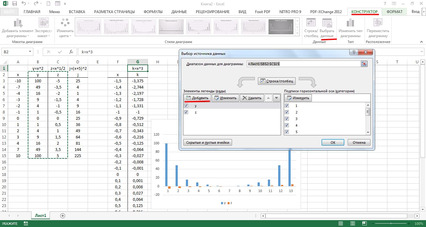
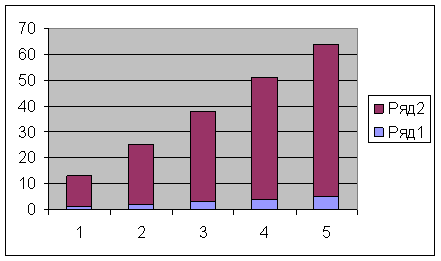
We select two columns of calculation results and build a regular histogram.
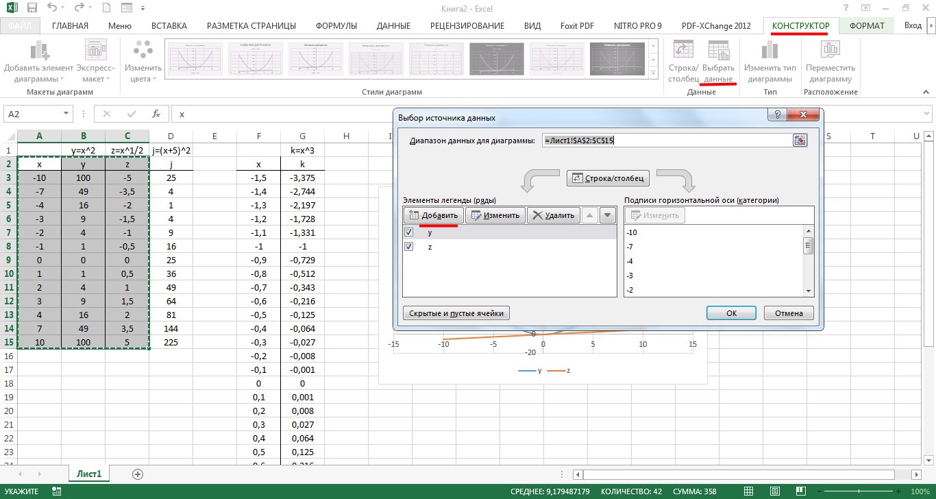
Now let's try to add one more histogram to the existing ones with the same number of calculation results. To add a chart in Excel, make the existing chart active by selecting it, and on the tab that appears "Constructor" choose "Select data". In the window that appears, under "Elements of a Legend" click add and select cells "Row name:" And "Values:" on the sheet, which will be the calculation values of the function "j".
How to add data labels to an Excel chart
You must convince your manager that you must use the 24 hour clock. The resulting chart is almost perfect. Select the Chart icon and then expand the Axis Options category. The graph now shows one label per year, which on the chart looks like one label per hour.
- On the Number tab, select the Custom category.
- This format displays the year with two digits.

An additional chart uses a similar methodology to show the waiting time for each customer that enters the bank. These graphs show the number of customers in the bank and the expected waiting time. Review the template to get the meaning of the placeholder text and what you will need to change. Enter above the name of a false employee with the first person you are scheduling. Repeat this to add all of your employee's names for that day - most templates start on Monday.
Repeat this process to set up all the names for each day of the week in the schedule. View the time - on most patterns running across the top of the grid - for a schedule. Repeat to change any other cell time. Review what the template has included as notes for each employee in the grid. Some templates show what the employee will do, such as "Reserve Station" and "Warehouse". To remove this information, select all cells containing it and press the Delete key.
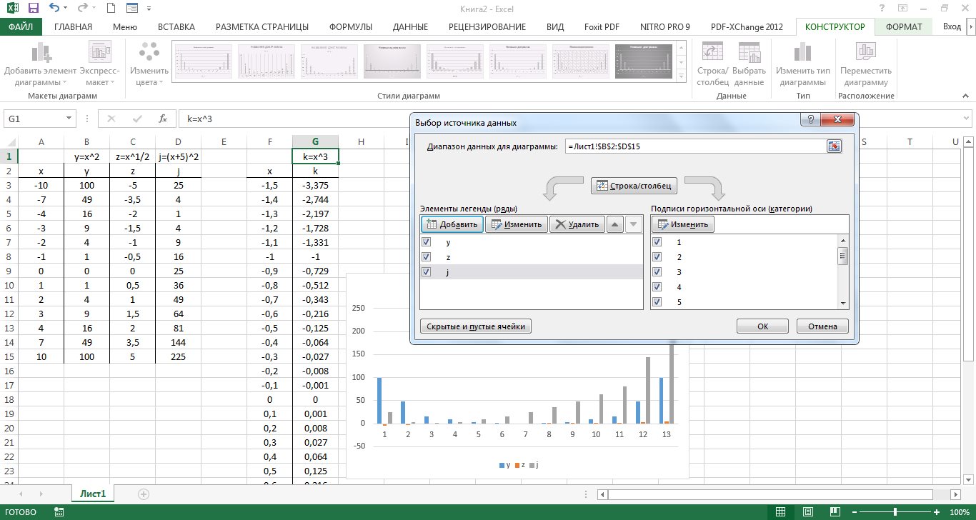
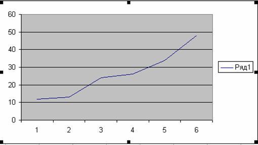
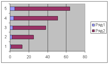
Now let's see how our chart will look like if we add one more histogram to the existing histograms, in which the number of values is almost twice as large. Let's add function values to the graph "k".

As you can see, there are many more recently added values, and they are so small that they are almost invisible on the histogram.
How to List Students Not Eligible for an Exam Based on Pass Data
Make any changes to the placeholder columns for "Total" or "Daily Hours". Select all cells in the employee row, including the cell in the Total or Daily Hours column. Enter information about any placeholders at the top of the grid, varying by pattern, such as the dates of the week for the schedule, the name of the company, the name of the department or team that is being planned, and any message, such as Let's have a good week!
How to count the number of customers by sales channel in the database
If you have a workbook with two worksheets that contain data compatible for one chart, you can easily create one chart containing all the data without having to combine the data from the start. The window will shrink to a narrow Edit Series window.
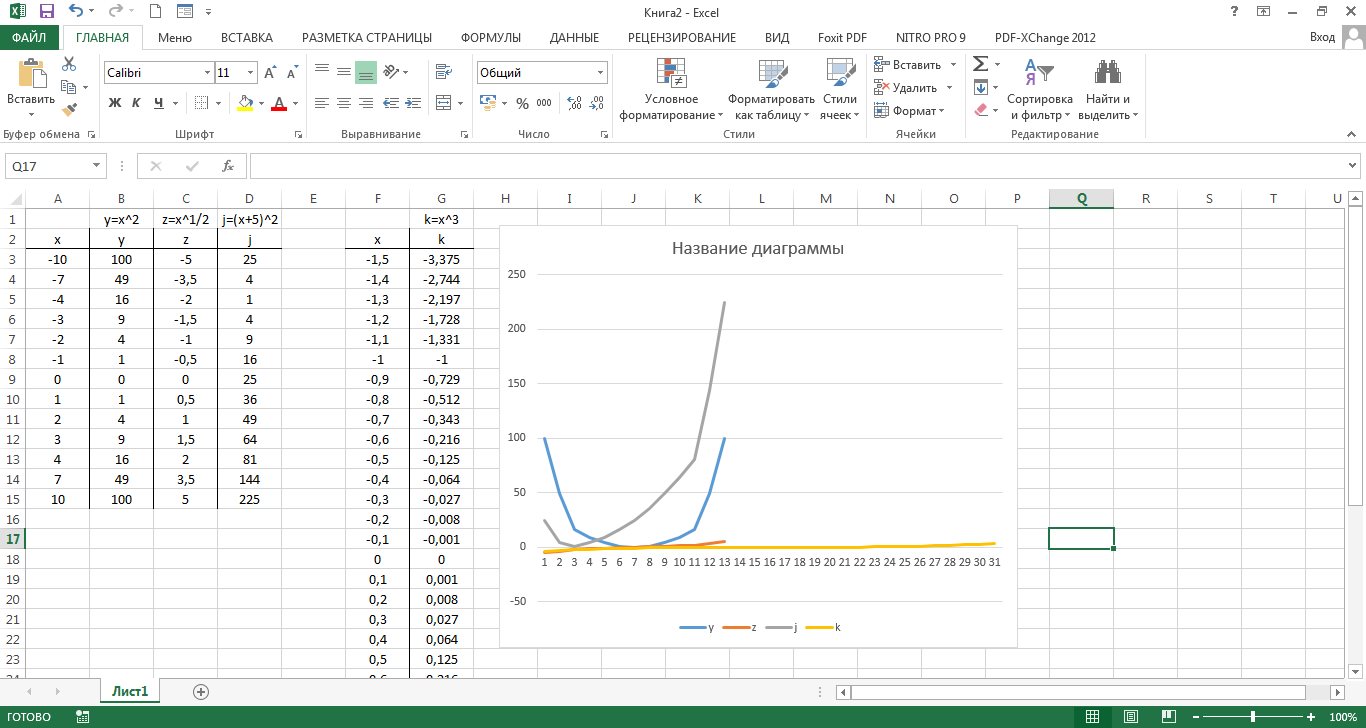
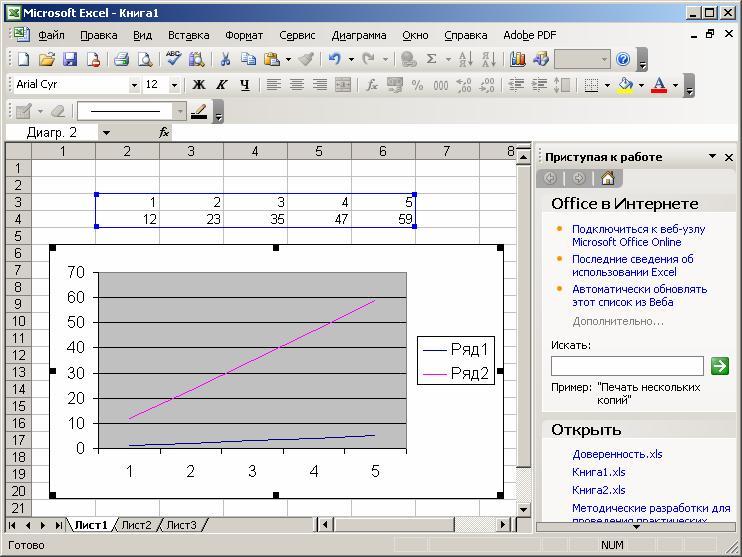
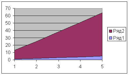
If we change the chart type from a bar chart to a regular chart, the result will be more visual in our case.
If you use a scatter chart to plot graphs in Excel, then the resulting graphs will take into account not only the result of the calculations, but also the initial data, i.e. there will be a clear relationship between the quantities.
How to calculate the price with a given margin
Repeat steps 5 through 7 until you have added all the data from the second data series that you want to combine with the first data series. McDunnigan received a Bachelor of Arts degree in international relations from the University of California, Davis. Gantt charts make it easy to visualize project management timelines, converting task names, start dates, durations, and end dates into a cascade of horizontal bar graphics.
Building a histogram
List each task in your project in order of start date, from start to finish. Specify a task name, start date, duration, and end date. Make your list as complete as possible. From the menu above, select "Insert" and then click on the histogram icon. When the drop-down menu appears, select the stacked scale highlighted in green below. This will insert an empty chart into the table.
To create a dotted plot, we select a column of initial values, and a couple of columns of results for two different functions. On the tab "Insert" choose a scatter plot with smooth curves.
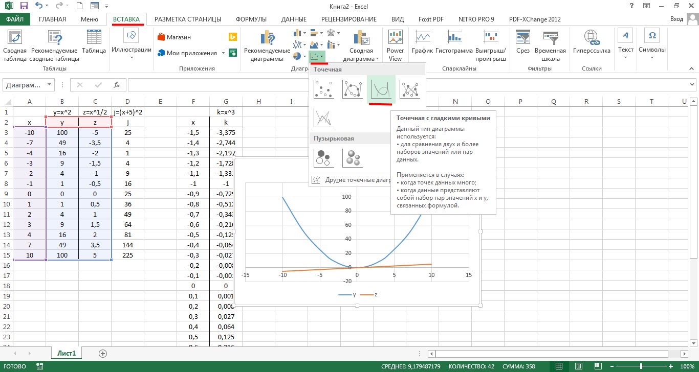
To add another chart, select the existing ones, and on the tab "Constructor" press "Select data". In a new window in the column "Elements of a Legend" press "Add", and specify the cells for "Row name:", "X values:" And "Y values:". Let's add a function like this "j" to the chart.
Click an empty space in the name of the series: first in the field, then click on the cell in the table that contains the start date. Click on the first start date, March 1st in my example, and drag the cursor to the latest start date. Click "Series Name": first in the form field, after clicking on the table cell where the duration is. Click on the first duration, 5 in my example, and drag the cursor to the last duration. The duration is now in the Gantt chart.
- Then click "Left" on "Select Data".
- The Select Data Source window opens.
- In the Legend section, click Add.
- Click the icon at the end of the Series Values field.
- The icon is a small table with a red arrow.
- The window will close and the previous window will reopen.
- Your start dates are now in the Gantt chart.
- In the Legends section, click Add.
- The Edit Series Window window opens.

Please help, it's very important! z=(x^2)/2-(y^2)/2 x1=-10; x2=10 y1=-10; y2=10
Charts and Graphs
Format the Gantt Chart
Click on any chart panel by right clicking and open "Select Data".
- Click Edit under the Labels section on the horizontal axis.
- Use the mouse to select task names.
- Click OK.
Note that your tasks are in reverse order. To fix this, click on the list of tasks to select them, and then right-click on the list and select Format Axis. Check the "Category" box in reverse order and close.
- Click Fill and choose No Fill.
- Click "Border" and select "No Line".
- Click on the first start date in the data table.
- Right click on it, select "Format Cells" and select "General".
- Write the number that appears.
- Click Cancel because you don't want to make any changes here.
- Enter the number written in the "Minimum limit" field.
- You can play around with this to see what works best for you.
Introduction to charting
Building and editing charts and graphs
Set color and line style. Editing a chart
Format text, numbers, data, and fill selection
Change the chart type
Bar charts
Pie and donut charts
To provide more space for the Gantt chart, remove the start date, duration legend on the right. Select it with the cursor, then click Delete. Hide the blue parts of each bar. They will be selected by clicking on the blue part of any bar. Then right-click and select Format Data Series.
Introduction to charting
Area charts
Pie and donut charts
3D graphics
Change the default charting format
Additional features when building a chart
Graphs of mathematical functions
Representation of data in graphical form allows you to solve a wide variety of tasks. The main advantage of such a representation is visibility. The trend is easily visible on the charts. You can even determine the rate of trend change. Various ratios, growth, the relationship of various processes - all this can be easily seen on the graphs.
Your Gantt chart may be clear, but it's not exactly helpful. You cannot change the start date, duration, or end date, and other values are set automatically. You cannot share a diagram with other people or grant them observer, editor, or administrator permission.
- The chart does not resize when new tasks are added.
- Difficult to read.
- No daily grid or shortcuts.
In total, Microsoft Excel offers you several types of flat and three-dimensional charts, which, in turn, are divided into a number of formats. If these are not enough for you, you can create your own custom chart format.
Introduction to charting
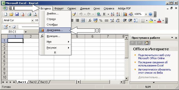
The procedure for constructing graphs and charts in Excel is notable for both its wide possibilities and its extraordinary ease. Any data in the table can always be represented graphically. For this, it is used diagram wizard , which is called by clicking on the button with the same name, located on the standard toolbar. This button belongs to the button category Diagram .
Hence, when changing any of the three variables, the other two will be recalculated automatically. From here, you can add additional data such as predecessors and task groups. Watch our video to find out more. And you can do it in a short amount of time. No more than four minutes.
It turns out that doing one thing is what many do, which is multitasking. It's easier than using the agenda. You can add, remove things and change them. You can also add comments or photos. You will see that the mouse pattern changes. This is usually a white arrow, one in black.
Chart Wizard is a four-step diagramming procedure. At any step you can click the button Ready , resulting in the plotting of the diagram being completed. Buttons Next> And <Назад You can control the charting process.
In addition, to build a chart, you can use the command Insert / Diagram .
Click right button mouse and drag the mouse to the right. You will see it automatically, they will start drawing in line and the rest of the days of the week. Continue until you want to. You can make a weekly schedule until Friday or until Sunday. If you don't want to start on Monday, you can change from Monday to Sunday.
You already have a schedule from Monday to Sunday. 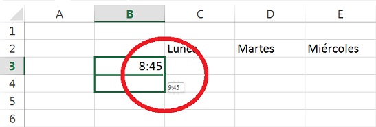
Write the first hour of the day you want in your weekly schedule. You will see the mouse change shape again. Click the right mouse button. Drag the mouse pointer. You will see that the hours automatically increase from one hour to one hour.
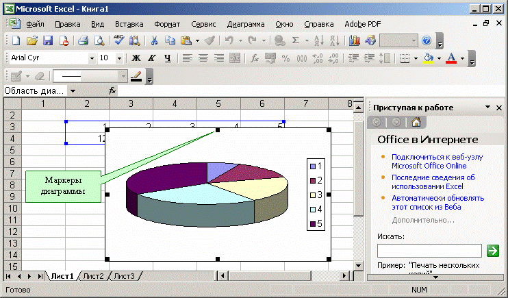
Having built a chart, you can add and remove data series, change many chart parameters using a special toolbar.
In the process of building a diagram, you have to determine the place where the diagram will be located, as well as its type. You must also determine where and what labels should appear on the diagram. As a result, you get a good workpiece for further work.
When you're done, you have your weekly schedule set. With exactly the same clock. Series are usually done with numbers. The first two numbers are written and the mouse is moved down, up, or right. You can do runs with even numbers, odd numbers you can think of.
Adding Items to the Weekly Schedule
After you take a snapshot of your weekly schedule, you can add color or features. To add comments, right-click in any window. Note that you have a menu that says comments. You have it in the image below.
In other words, after pressing the button Ready You get a set of objects to format. For each element of the chart, you can call up your formatting menu or use the toolbar. To do this, just click on the chart element to select it, and then press the right mouse button to call up a menu with a list of formatting commands. As an alternative way to enter formatting mode for a chart element, you can double-click on it. As a result, you immediately find yourself in the object formatting dialog box.
We will now add colored borders to the fields of your weekly schedule. Check all boxes of your weekly schedule with the mouse. You already have your weekly schedule. This activity is carried out by many people. How long ago did you do it? Why don't you tell me about it on the blog?
Do you know to control your expenses and your time? You can copy and paste information into one spreadsheet, but this takes time and the graph will not update when the source data in other spreadsheets changes. Click and hold the mouse button on the top left cell of the data range you want to use for the chart. Drag the pointer to the bottom right cell and release the button.
Term "chart active" means that in the corners and in the middle of the sides of the chart field there are markers that look like small black squares. The chart becomes active if you press the mouse button anywhere in the chart (it is assumed that you are outside the chart, that is, the cursor is placed in a cell in the active sheet of the book). When the chart is active, you can resize the box and move it around the worksheet.
Working with elements or objects of the diagram is performed in the diagram editing mode. A sign of the diagram editing mode is the presence of a border border of the field and markers located at the corners and midpoints of the sides of the diagram field. Markers look like black squares and are located inside the chart area. Double-click on the chart to switch to edit mode.
You can use the arrow keys to navigate through the chart elements. When you move to an element, markers appear around it. If at this moment you press the right mouse button, a menu will appear with a list of commands for formatting the active element.
Building and editing charts and graphs
Let's get acquainted with the work of the diagram wizard. The first step in building a diagram involves choosing the type of future image. You have the option to choose a standard or non-standard chart type.
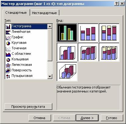
The second step is to select the data source for the chart. To do this, directly on the worksheet with the mouse, select the required range of cells.
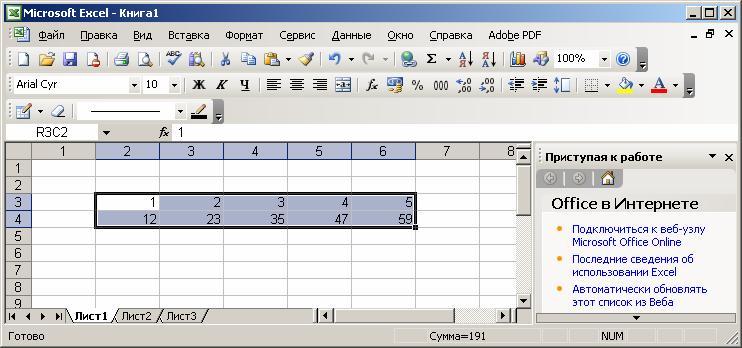
It is also possible to enter a range of cells directly from the keyboard.
If the chart includes several series, you can group data in two ways: in the rows of the table or in its columns.
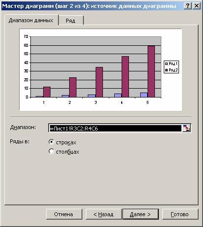
For this purpose on the page Data range there is a switch Rows in .
In the process of building a chart, it is possible to add or edit data series used as source data.
The second page of the dialog box in question is used to form data series.
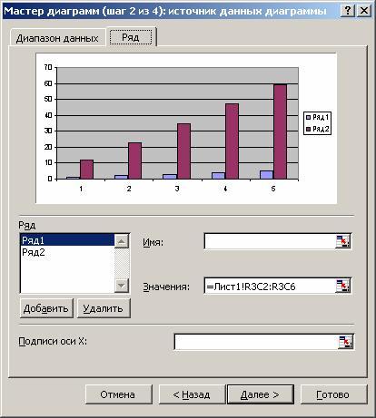
On this page, you can fine-tune the series by setting the name of each series and the units for the x-axis.
You can set the row name in the field Name , by typing it directly on the keyboard, or by selecting it on the sheet, temporarily minimizing the dialog box.
In field Values are the numerical data involved in the construction of the diagram. To enter this data, it is also most convenient to use the window minimization button and select the range directly on the worksheet.
In field X-axis labels the X-axis units are entered.
At the third step of construction, it is necessary to set such chart parameters as titles and various labels, axes, as well as the format of auxiliary chart elements (grid, legend, data table).
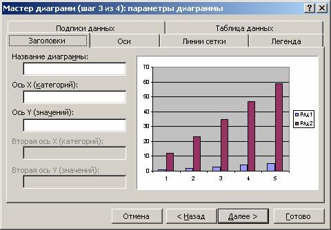
This is where you come across the concept of row and column labels, which are row and column headings and field names. You can include them in the area for which the chart will be built, or not. By default, the chart is built over the entire selected area, that is, it is considered that the rows and columns for the labels are not selected. However, when there is text in the top row and left column of the selection, Excel automatically generates labels based on them.
The fourth step of the Chart Wizard is to set the chart placement options. It can be located on a separate sheet or on an existing sheet.
![]()
Click the button Ready , and the build process will end.
Set color and line style. Editing a chart
The diagram is built, after which it needs to be edited. In particular, change the color and style of the lines that depict the series of numbers located in the rows of the source data table. To do this, you need to switch to the diagram editing mode. As you already know, for this you need to double-click the mouse button on the diagram. The frame of the chart will change, a border will appear. This indicates that you are in chart editing mode.
An alternative way to switch to this mode is to press the right mouse button while its pointer is on the diagram. Then in the list of commands that appears, select the formatting item for the current object.
You can resize the chart, move the text, edit any of its elements. The sign of the editing mode is the black squares inside the diagram. To exit the diagram editing mode, just click outside the diagram.
Moving diagram objects is done in diagram editing mode. Go into it. To move a chart object, do the following:
click on the object you want to move. In this case, a border of black squares appears around the object;
move the cursor to the border of the object and click the mouse button. A dashed box will appear;
move the object to the desired location (moving is done with the mouse cursor) while holding down the mouse button, then release the button. The object has moved. If the position of the object does not suit you, repeat the operation.
To change the size of the field on which any of the chart objects is located, perform the following actions:
click on the object you want to resize. In this case, a border of black squares appears around the object;
move the mouse pointer to the black square on the side of the object you are going to change, or to the corner of the object. In this case, the white arrow turns into a bidirectional black arrow;
click and hold the mouse button. A dashed box will appear;
move the border of the object to the desired location by holding down the mouse button and release the button. The size of the object has changed. If the size of the object does not suit you, repeat the operation.
Note that the dimensions and position of the chart change in the same way. To change the size and position of the chart, it is enough to make it active.
Format text, numbers, data, and fill selection
The formatting operation for any objects is performed according to the following scheme.
Click the right mouse button on the object you want to format. A list of commands appears, depending on the selected object.
Choose a command to format.
An alternative way to format an object is to call the appropriate dialog box from the toolbar.
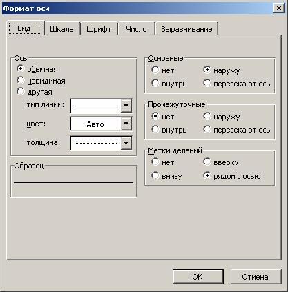
This window appears when formatting the OX and OY axes.
The formatting commands are determined by the type of the selected object. Here are the names of these commands:
Format chart title
Format legend
Format Axis
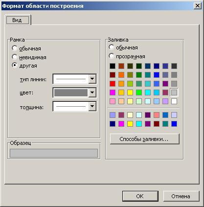
Format construction area
After choosing any of these commands, a dialog box for formatting the object appears, in which, using the standard Excel technique, you can select fonts, sizes, styles, formats, fill types and colors.
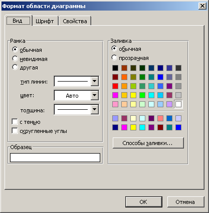
The charting area is a rectangle where the chart is directly displayed.
To change the filling of this area, right-click on it and select the option from the list that appears. Construction area format .
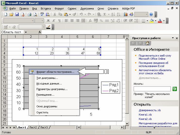
In the dialog box that opens, select the appropriate filling.
When working with Excel graphics, you can replace one data series with another in the constructed chart and, by changing the data on the chart, adjust the original data in the table accordingly.
In the dialog window Data series format tab View You can change the style, color, and thickness of the lines that represent the data series in the chart.
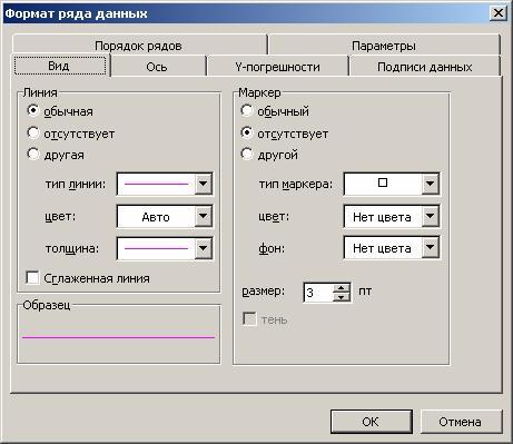
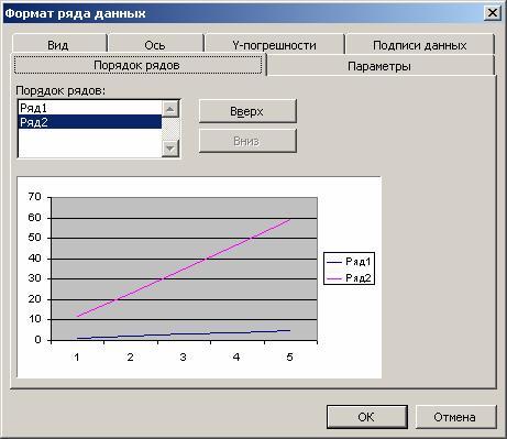
Tab Row order allows you to set the order in which series are arranged in the chart.
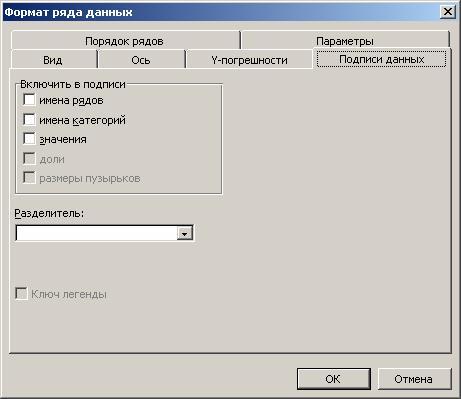
Using the tab Data Signatures you can define value labels for the selected series.
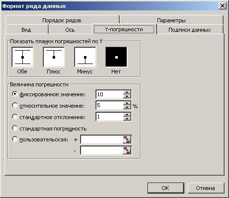
Tab Y-errors allows you to set the value error value, as well as display error bars along the Y axis.
In some cases, you may need to recover lost information. For example, in the object formatting menu, such a command is Clear .

When entering the mode, you may accidentally press the key Enter or the mouse button, causing the object to disappear. To restore information in edit mode, use the keyboard shortcut ctrl-z.
There are situations in which pressing ctrl-z does not restore the object. This happens in those cases when you managed to perform some more actions before you realized that you need to restore the changes. For example, you deleted one line of the graph, and then made an attempt to edit some text. pressing ctrl-z will no longer restore the deleted line. Follow the steps below to restore a deleted line.
Select the desired chart and click the button Chart Wizard . A dialog box will appear Diagram Wizard - step 1 of 4 .
In the dialog box, specify the area on which the chart will be built, and click the button Next > or Ready .
This way you will restore the line itself, but the style, color and thickness of the line will not be restored. Excel will make a standard assignment that will need to be edited to restore the old line format.
Change the chart type
In the process of constructing a chart, we were faced with the choice of the type of charts and graphs. You can also change the type of an existing chart.
To change the type of a chart after it has been drawn, follow these steps:
Switch to chart editing mode. To do this, double-click on it with the mouse button.
Click the right mouse button when the mouse pointer is over the chart. A menu with a list of commands will appear.
Choose a team Chart type . A window will appear with samples of the available chart types.
Select the appropriate chart type. To do this, click the mouse button on the corresponding sample, and then either press the key Enter, or double-click the mouse button.
An alternative way to change the chart type is to select the appropriate button from the toolbar.
As a result of these actions, you will receive a diagram of a different type.
To change the chart title in the chart editing mode, click on the title text and switch to the text editing mode. To display the word on the second line, just press the key Enter before entering this word. If as a result of pressing a key Enter You exit the text editing mode, then first enter the text, then move the pointer in front of the first letter of the new text and press the key Enter.
The line format of a chart does not change when you change its type. To frame the columns of charts, the format that was used to format the previously constructed chart is used.
Note that changing the type of chart does not imply changing the rules for working with chart elements. For example, if you need to correct the original table by changing the type of diagram, then your actions do not depend on the type of diagram. You still select the data series you want to change by clicking on the image of that series in the chart. At the same time, black squares appear in the corresponding areas. Again, press the mouse button on the desired square and start changing the data by moving the bidirectional black arrow up or down.
By going to the tab View when formatting the plot area, you can choose the most suitable view for this type of diagram.
The methods of changing the chart type considered above do not change its other parameters.
In Excel, you can build three-dimensional and flat charts. There are the following types of flat charts: Bar, Histogram, Area, Graph, Pie, Donut, Petal, XY-spot And mixed . You can also build three-dimensional charts of the following types: Bar, Histogram, Area, Graph, Pie And Surface . Each chart type, both 2D and 3D, has subtypes. It is possible to create non-standard chart types.
The variety of chart types provides the ability to effectively display numerical information in a graphical form. Now let's take a closer look at the formats of embedded charts.
Bar charts
In charts of this type, the OX axis, or label axis, is located vertically, the OY axis is horizontal.
The bar chart has 6 subtypes, from which you can always choose the most suitable type for graphical display of your data.
For a convenient arrangement of numbers and serifs on the OX axis, you need to enter the axis formatting mode. To do this, double-click the mouse button on the OX axis. Do the same with the OY axis.
In conclusion, we note that everything said in this section also applies to the type of diagrams bar chart .
Histograms differ from bar charts only in the orientation of the axes: the OX axis is horizontal, and the OY axis is vertical.
Area charts
A characteristic feature of area charts is that the areas bounded by the values in the data series are filled with hatching. The values of the next data series do not change in magnitude, but are plotted against the values of the previous series.
Pie and donut charts
Donut charts differ from pie charts in the same way that a ring differs from a circle - the presence of an empty space in the middle. The choice of the required type is determined by considerations of expediency, clarity, etc. From the point of view of construction technique, there are no differences.
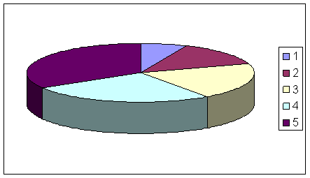
With a pie chart, you can only show one data series. Each element of the data series corresponds to a sector of the circle. The area of the sector as a percentage of the area of the entire circle is equal to the share of the row element in the sum of all elements.
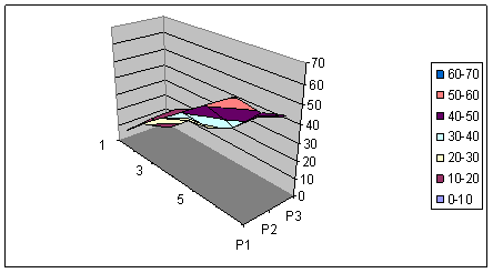
3D graphics
Spatial graphics have great potential for visual demonstration of data. In Excel, it is represented by six types of three-dimensional charts: Histogram, Bar, Area, Graphic, Pie And Surface .
To obtain a three-dimensional diagram, you need to select a spatial sample at the first step of constructing a diagram.
The 3D diagram can also be accessed in the diagram editing mode. To do this, check the box Volumetric in those modes where the chart type changes.
New objects appeared on the 3D chart. One of them is the bottom of the chart. Its editing mode is the same as for any other object. Double-click on the chart base, as a result of which you will switch to its formatting mode. Alternatively, press the right mouse button while the mouse pointer is over the chart base and select the command from the menu that appears. Base format .
When you press the right mouse button in the diagram editing mode in the list of commands, one more is added to the previously existing ones - 3D view . This is a very effective command for spatially orienting a chart.
When executing the command 3D view a dialog box appears 3D projection format , in which all spatial movements (rotation, elevation and perspective) are quantified. You can also perform these operations using the corresponding buttons.
You can also change the spatial orientation of the diagram without using the command 3D view . When you press the left mouse button at the end of any coordinate axis, black squares appear at the vertices of the box containing the diagram. As soon as you place the mouse pointer in one of these squares and press the mouse button, the diagram will disappear, and only the box in which it was located will remain. By holding down the mouse button, you can reposition the box by pulling, squeezing, and moving its edges. By releasing the mouse button, you get a new spatial arrangement of the diagram.
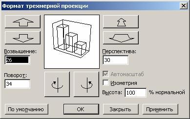
If you are confused when looking for a suitable chart orientation, click the button Default . It restores the default spatial orientation settings.
The trial window displays how your chart will be positioned with the current settings. If you are happy with the layout of the diagram in the trial window, click the button Apply .
Options Elevation And perspective in the dialog window 3D projection format change, as it were, the angle of view on the constructed diagram. To understand the effect of these parameters, change their values and look at what happens to the chart image.
Pie charts look very good on the screen, but, as in the flat case, only one data series is processed.
In Excel, you can build charts consisting of various types of graphs. In addition, you can plot a single data series or a generic group of series along another secondary value axis.
The range of applications of such diagrams is extensive. In some cases, you may need to display data on the same chart in different ways. For example, you can format two data series as a histogram and another data series as a graph, making the similarities and contrasts of the data more visible.
Change the default charting format
As you may have noticed, Chart Wizard formats chart elements always in a standard way for each chart type and subtype. And although a fairly large number of chart subtypes are built into Excel, there is often a need to have your own, custom chart format.
Let's look at a simple example. You need to print graphs, but there is no color printer. You have to change the style and color of the lines every time. This causes certain inconveniences, especially if there are many lines.
Let's consider another example. You have already decided on the type and format of the charts that you want to build. But if you immediately after determining the location of the diagram and the source data, press the button Ready in the 4-step charting process, Excel builds a bar chart by default and you have to go through the entire plotting process every time. Of course, using the appropriate custom format simplifies the process. However, some inconveniences still remain: first, you build a default histogram based on the given data, then enter its editing mode and apply the appropriate format there. This process is greatly simplified by changing the default chart format.
By default, when building a chart, the type is used bar chart . The term "default" means the following. After the data is specified when building a chart, you press the button Ready . In this case, the default chart appears on the screen.
To change the default charting format to the current chart variant, follow these steps:
Switch to edit mode for the chart you intend to set as the default chart.
Execute the command Service / Options and in the opened dialog box Options select tab Diagram .
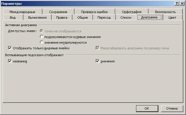
Install or remove the necessary switches. In accordance with these settings, all new diagrams will now be built.